Einführung

In den vorangegangenen Posts haben wir zu einem einfachen linearen Regressionsmodell \(\hat{Y}=i_Y + cX\) eine weitere Variable hinzugefügt, die die Position eines Mediators \(M\) oder Moderators \(W\) eingenommen hat. Es ergaben sich dadurch folgende Modelle in ihrer je einfachsten Form:

Moderator-Modelle:

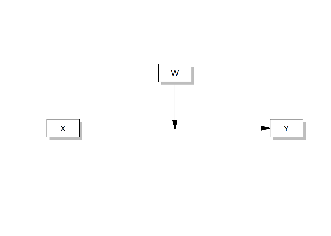
Eine Gleichung (multiple Regression + gewichtetem Interaktionsterm) \[ \small \begin{align*} \hat{Y} = i_Y + b_1X + b_2W + b_3XW \\ = i_Y + (b_1 + b_3W)X + b_2W \end{align*} \]

Mediator-Modelle:

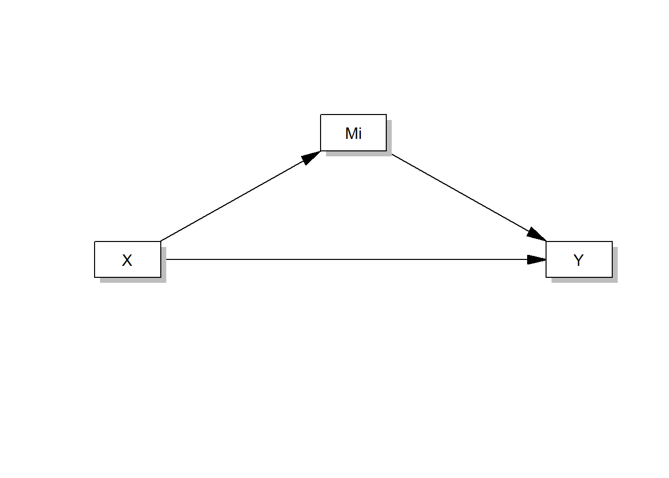
Zwei Regressionsgleichungen für (Mediator und abhängige Variable) \[ \small \begin{align*} \hat{M} & = i_M + aX \\ \hat{Y} & = i_Y + c'X + bM \end{align*} \]

Conditional Process Model

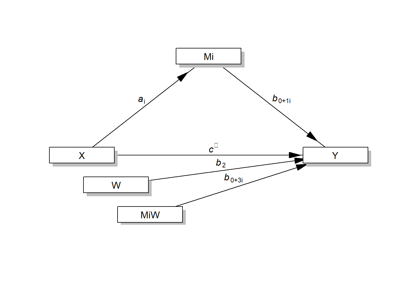
Es ist naheliegend diese beiden Modelle in einem zu verbinden. Dieses gemeinsame Modell wird als Conditional Process Model bezeichnet (Bedingte Prozessanalyse).

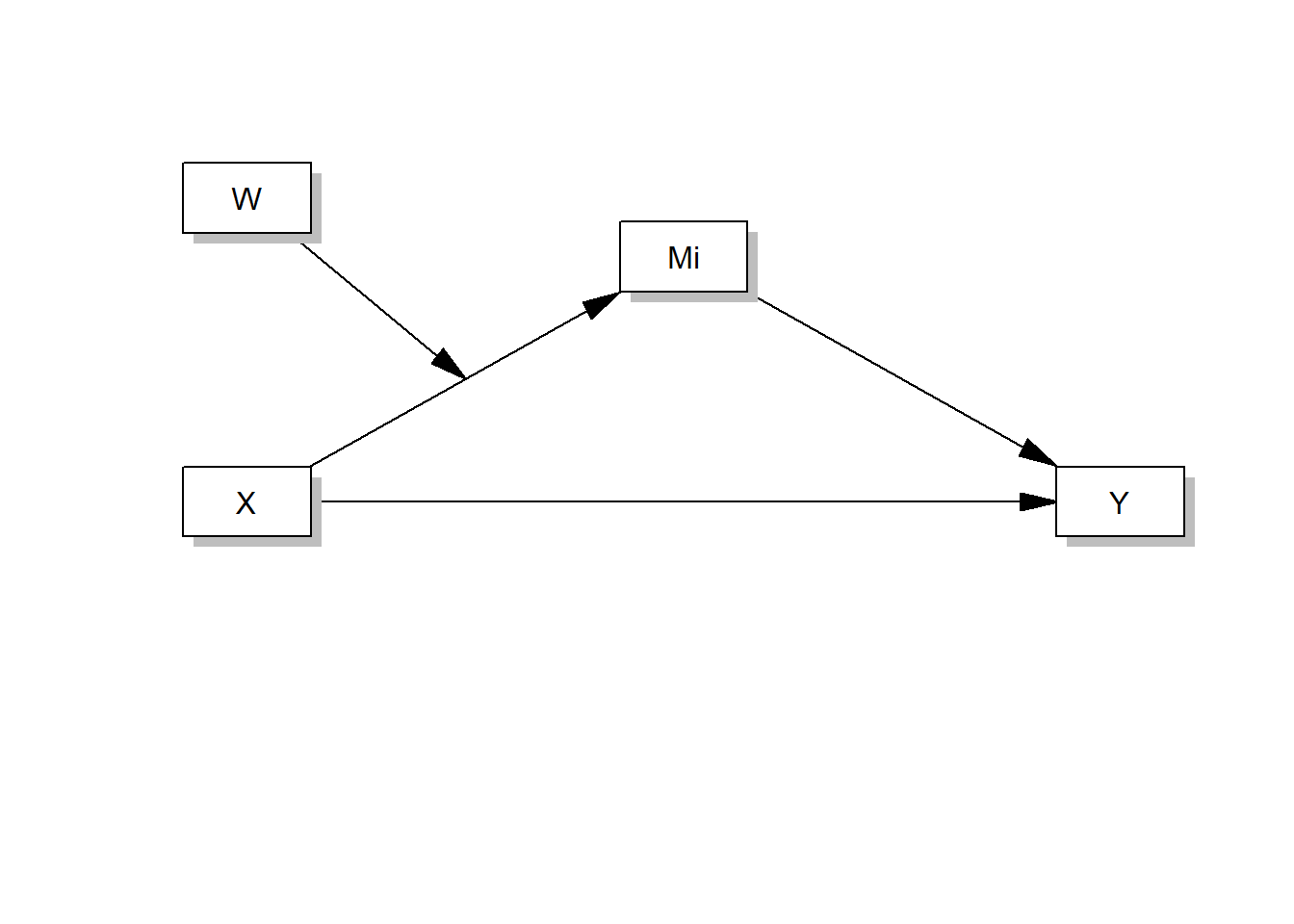
Es ergeben sich für dieses einfache Modell folgende zwei Gleichungen: \[ \small \begin{align*} \hat{M} = i_M + a_1X + a_2W + a_3XW \\ = i_M + (a_1 + a_3W)X + a_2W \end{align*} \] und \[ \small \begin{align*} \hat{Y} = i_Y + c_1'X + c_2'W + c_3'XW + bM \\ = i_Y + (c'_1+c'_3W)X + c'_2W + bM \end{align*} \]

Pakete

library(magrittr)
library(dplyr)
library(tidyr)
library(haven)
library(here)

library(processR)
library(lavaan)

library(ggplot2)
library(ggpmisc)

Übungsaufgaben

Aufgabe 1

Hayes (2022, Abschn. 11.3) diskutiert eine Studie von Cole et al. (2008), in welcher Daten von 60 Arbeitsgruppen einer Firma, welche Autoersatzteile herstellt, erhoben wurden. Die sog. experimentellen Einheiten dieser Untersuchung sind also Gruppen, nicht Individuen. Die folgenden vier Variablen liegen vor:

dysfunc: Der Grad der Dysfunktionalität während der Zusammenarbeit in der Gruppe. In Arbeitsgruppen mit hohen dysfunc-Werten behindern sich Mitglieder gegenseitig, verhindern Innovation, usw.
negtone: Ein Indikator für die Schlechtigkeit des Arbeitsklimas innerhalb der Gruppe (Grad negativer Gefühle).
perform: Die Produktivität der Zusammenarbeit.
negexp: Die Sichtbarkeit des negativen Arbeitsklimas aufgrund nicht-verbaler Hinweise.

Das Ziel der Studie war, den Mechanismus zwischen diesem beiden Variablen zu analysieren. Dazu wurden zwei Annahmen gemacht, die insofern einer kausalen Theorie entsprechen, als sie jeweils einer Variablen die Rolle des Mediators bzw. des Moderators zuweisen.

Die Schlechtigkeit des Arbeitsklimas wird als Mediator betrachtet, welcher den Effekt der Dysfunktionalität auf die Produktivität vermittelt.
Es wird vermutet, dass eine geringere Sichtbarkeit des negativen Arbeitsklimas, zur Aufrechterhaltung der Produktivität der Arbeitsgruppe beiträgt. Mit anderen Worten, Sichtbarkeit moderiert den Effekt des Arbeitsklimas auf die Produktivität.

Zeichnen Sie ein konzeptuelles Diagramm der vier Variablen.
Berechnen Sie deskriptive Kennwerte (Mittelwert und Standardabweichung).
Formulieren Sie sowohl das Modell des Mediators sowie das Modell der Produktivität.
Berechnen Sie die beiden Modellgleichungen mit zwei Regressionsmodellen.
Wie wird die Steigung des Modells für den Mediator interpretiert? Ist diese Steigung signifikant?
Ist negexp ein Moderator.
Wie werden die Steigungen von \(M\) und \(W\) interpretiert?
Anstatt die \(b_3\) Steigung direkt zu interpretieren, betrachtet man den bedingten Effekt des negativen Arbeitsklimas auf die Produktivität, der eine Funktion der Sichtbarkeit ist. Wie lautet dieser bedingte Effekt.
Um den bedingten Effekt besser zu verstehen, wird er für einen kleinen, mittleren und großen Wert des Moderators berechnet. Hayes schlägt vor, die bedingten Effekte des 16., 50. und 84. Perzentils zu verwenden. Fertigen Sie einen Simple-Slopes-Plot an. Dafür müssen zunächst die Steigungen und Konstanten der drei Geraden berechnet werden. Anschließend wird ein Streudiagramm von Arbeitsklimas und Produktivität angefertigt, in das die drei Geraden eingezeichnet werden.
Von inhaltlichem Interesse ist die Größe der bedingten indirekten Effekte. Für das aktuelle Modell ergeben sich diese als das Produkt von \(a\) mit den bedingten direkten Effekten.
Wie wird der direkte Effekt \(c′\) der Dysfunktionalität auf Produktivität interpretiert?

Erläuterung

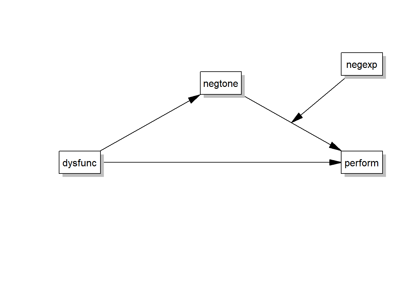
In der Originalarbeit findet sich in dem Beispiel Hiding Your Feelings from Your Work Team folgende Formulierung (Hayes, 2022, S. 422–423):

according to research on teamwork by Cole et al. (2008) sometimes it may be better to hide your feelings from others you work with about the things they do or say that bother you, lest those feelings become the focus of attention of the team and thereby distract the team from accomplishing a task in a timely and efficient manner.

The study involved 60 work teams employed by an automobile parts manufacturing firm and is based on responses to a survey from over 200 people at the company to a series of questions about their work team […]. Four variables that are pertinent to this analysis were measured. Members of the team were asked a series of questions about the dysfunctional behavior of members of the team, such as how often members of the team did things to weaken the work of others or hinder change and innovation (dysfunc: higher scores reflect more dysfunctional behavior in the team). The negative affective tone of the group was also measured by asking members of the team how often they felt “angry”, “disgusted”, and so forth, at work (negtone: higher scores reflecting a more negative affective tone of the work environment). The team supervisor was asked to provide an assessment of team performance in general, such as how efficient and timely the team is, whether the team meets its manufacturing objectives, and so forth (perform: scaled with higher values reflecting better performance). In addition, the supervisor responded to a series of questions gauging how easy it is to read the nonverbal signals team members emote about how they are feeling – their nonverbal negative expressivity (negexp: higher scores meaning the members of the team were more nonverbally expressive about their negative emotional states). This goal of the study was to examine the mechanism by which the dysfunctional behavior of members of a work team can negatively affect the ability of a work team to perform well. They proposed a mediation model in which dysfunctional behavior (\(X\)) leads to a work environment filled with negative emotions (\(M\)) that supervisors and other employees confront and attempt to manage, which then distract from work and interfere with task performance (\(Y\)). However, according to their model, when team members are able to regulate their display of negative emotions (\(W\)), essentially hiding how they are feeling fromothers, this allows the team to stay focused on the task at hand rather than having to shift focus toward managing the negative tone of the work environment and the feelings of others. That is, the effect of negative affective tone of the work environment on team performance is hypothesized in their model as contingent on the ability of the team members to hide their feelings from the team, with a stronger negative effect of negative affective tone on performance in teams that express their negativity rather than conceal it.

Daten

df_proc <- haven::read_sav(here("data", "proc", "teams.sav")) %>% 
           haven::zap_formats() %>% 
           haven::zap_labels()

Teilaufgaben

Teilaufgabe a

Zeichnen Sie ein konzeptuelles Diagramm der vier Variablen.

Teilaufgabe b

Berechnen Sie deskriptive Kennwerte (Mittelwert und Standardabweichung).

df_proc %>% summarise_all(.funs = list(M = mean, SD = sd))

variable	M	SD
dysfunc	0.03	0.37
negexp	-0.01	0.54
negtone	0.05	0.53
perform	-0.03	0.52

Anmerkung. Die Daten sind im Mittel alle nahe null, i.e. null sofern gerundet auf eine Nachkommastelle.

Teilaufgabe c

Formulieren Sie sowohl das Modell des Mediators sowie das Modell der Produktivität.

Es ergeben sich folgende Modellgleichungen

Modell des Mediators: \(M = i_M + aX + e_n\)
Modell der Produktivität: \(Y = i_Y + c'X + b_1M + b_2W + b_3MW\)

Teilaufgabe d

Berechnen Sie die beiden Modellgleichungen mit zwei Regressionsmodellen.

# lm mediator M
mdl_m <- lm(negtone ~ dysfunc, data = df_proc)
# lm dv
mdl_dv <- lm(perform ~ dysfunc + negtone + negexp + negtone:negexp, 
             data = df_proc)

Teilaufgabe e

Wie wird die Steigung des Modells für den Mediator interpretiert? Ist diese Steigung signifikant?

summary(mdl_m)

term	b	SE	t	p
(Intercept)	0.026	0.062	0.416	.7
dysfunc	0.620	0.167	3.715	<.001

Je dysfunktionaler die Arbeitsgruppe arbeitet (dysfunc), desto negativer ist die Stimmunglage (negtone) aka. desto schlechter das Arbeitsklima. Konkrete geht eine Erhöhung der Dysfunktionalität um eine Einheit mit einer Verschlechterung der Stimmungslage um \(a = .62\) einher. Diese Steigung \(b\) ist signifikant (vgl. \(p < .001\)).

Teilaufgabe f

Ist negexp ein Moderator?

summary(mdl_dv)

term	b	SE	t	p
(Intercept)	-0.012	0.059	-0.203	.84
dysfunc	0.366	0.178	2.059	.04
negtone	-0.436	0.131	-3.338	<.01
negexp	-0.019	0.117	-0.163	.87
negtone:negexp	-0.517	0.241	-2.146	.04

Ja, das negative Arbeitsklima \(W\) ist eine Moderatorvariable (vgl. Interaktionsterm mit \(p < .05\)).

Teilaufgabe g

Wie werden die Steigungen von M und W interpretiert?

In \[ \begin{align*} Y & = i_Y + c'X + b_1M + b_2W + b_3MW \\ & = -0.012 + 0.366X-0.436M-0.019W-0.517MW \end{align*} \] setzen wir i) \(W=0\) um \(M\) bzw. dessen Steigung \(b_1\) interpretieren zu können und ii) vice verse \(M=0\) für \(W\) bzw. die Steigung \(b_2\). Da es sich bei null um die Mittelwerte (gerundet) der entsprechenden Variablen handelt, ist eine inhaltliche Interpretation möglich.

i) \(b_1\) (mit W = 0)

Durch W = 0 verschwindet sowohl \(b_2\) als auch der Interaktionsterm mit \(b_3\). Die verbleibende Gleichung lautet (vereinfacht ohne Fehlerterm):

\[Y = i_Y + c'X + b_1M\] \(b_1\) schätzt die Auswirkung des negativen Arbeitsklimas (negtone) in Teams auf deren Arbeitsleistung (perform) für jene Teams mit zum Durchschnitt grob gleich negativen Emotionen (negexp \(\approx 0\)) und gleichstark ausgeprägtem dysfunktionalen Verhalten (dysfunc = konstant). Dieser Effekt ist negativ und statistisch von Null verschieden, \(b_1 = -0,436\); \(p = .002\). Konkret geht eine Verschlechterung des Arbeitsklimas um eine Einheit mit einem Rückgang der Produktivität um \(0.436\) Einheiten (= Verschlechterung) einher und zwar für jene Teams mit durchschnittlicher negativer Emotionalität bei gleichzeitig dysfunktionalen Verhalten auf vergleichbarem Niveau.

Dazu schreibt Hayes (2022, S. 325):

\(b_1\) estimates the effect of negative affective tone on team performance in teams measuring zero in negative emotional expressivity but equal in dysfunctional behavior. This effect is negative and statistically different from zero, \(b_1 = -0.436\); \(p = .002\). This is substantively meaningful because zero is within the bounds of measurement in this study. A score of zero on nonverbal negative expressivity does not mean an absence of expressivity. Rather, zero is just barely above the sample mean (\(\bar{W}=-0.008\)). So holding constant dysfunctional behavior, among teams just slightly above average in expressivity, those functioning in a relatively more negative emotional climate are perceived by their supervisors as performing relatively less well.

Aja, dann hätten wir das also auch geklärt. Danke für nichts, Andrew 😒.

ii) \(b_2\) (mit M = 0)

Analog kann \(b_2\) interpretiert werden, durch Nullsetzten von M:

\[Y = i_Y + c'X + b_2W\]

\(b_2\) ist also der Grad, in dem sich negative Emotionen in Teams auf deren Arbeitsleistung auswirken, sofern es sich um Teams handelt, in denen ein durchschnittsähnliches negatives Arbeitsklima vorherscht (negton \(\approx 0\)) und die vergleichbares dysfunktionales Verhalten (dysfunc = konstant) zeigen. Allerdings ist \(b_2=-0.019\) nicht signifikant von null verschieden, \(p=.87\). Für den Fall eines bedeutsamen Zusammenhangs würde eine Verschlechterung der negativen Emotionen um eine Einheit mit einer Abnahme der Produktivität um 0.019 Einheiten einhergehen, sofern dabei Teams betrachtet werden, in denen das Arbeitsklima im Durchschnitt ungefähr gleich negativ ist und die dabei dysfunktionales Verhalten auf vergleichbar schlechtem Niveau zeigen.

The regression coefficient for nonverbal negative expressivity, \(b_2\), estimates the effect of nonverbal negative expressivity on team performance among teams measuring zero in negative affective tone. Zero is within the bounds of measurement and is just below the sample mean (\(\bar{M}=0.047\)). So among teams equal in dysfunctional behavior and slightly below the mean in negative affective tone, those teams whose members are more inclined to express their negative emotions perform less well. However, this effect is not statistically different from zero, \(b_2 = -0.019\); \(p = 0.871\).

Andrew auch hier wieder ganz genau unterwegs und selbstverständlich hat er Recht! Der Durchschnitt ist eben nicht genau null und um die Sakala überhaupt richtig interpretieren zu können, müssten wir uns die Studie von Cole et al. (2008) genauer ansehen. Ansonsten könnten wir aber auch Daten simulieren und damit überprüfen, wie wahrscheinlich es ist, dass der Mittelwert tatsächlich null ist (dazu aber mehr zu einem späteren Zeitpunkt).

Teilaufgabe h

Anstatt die \(b_3\) Steigung direkt zu interpretieren, betrachtet man den bedingten Effekt des negativen Arbeitsklimas auf die Produktivität, der eine Funktion der Sichtbarkeit ist. Wie lautet dieser bedingte Effekt.

\[y = i_y + c'X + (b_1+b_3W)M+ b_2W + e_y\]

\[ \begin{align*} \theta_{M\rightarrow y} & = b_1 + b_3 W \\ & = -0.436 - 0.517 \times W \\ & = -0.953 \times W \end{align*} \]

mdl_coef <- mdl_dv %>% 
            summary() %>% 
            coef() %>% 
            data.frame() %>% 
            select(Estimate) %>% 
            pull(Estimate)

Teilaufgabe i

Um den bedingten Effekt besser zu verstehen, wird er für einen kleinen, mittleren und großen Wert des Moderators berechnet. Hayes schlägt vor, die bedingten Effekte des 16., 50. und 84. Perzentils zu verwenden. Fertigen Sie einen Simple-Slopes-Plot an. Dafür müssen zunächst die Steigungen und Konstanten der drei Geraden berechnet werden. Anschließend wird ein Streudiagramm von Arbeitsklimas und Produktivität angefertigt, in das die drei Geraden eingezeichnet werden.

Steigung: \(\theta_{M\rightarrow y} = b_1 + b_3 W = -0.436 - 0.517 \times W\)
Y-Achsenabschnitt: \(i_y + c'\bar{X} + b_2W\)

Berechnung der drei Steigungen (Slopes) und zugehörigen Konstanten (Intercept)

df_proc %>% summarise(mean = mean(dysfunc),
                      W = quantile(negexp, c(.16, .50, .84))) %>% 
            mutate(label = ordered(W, levels = W, 
                                   labels = paste(c("Low", "Moderate", "High"), 
                                                  "expressivity")),
                   b0 = mdl_coef[1],
                   c_ = mdl_coef[2],
                   b1 = mdl_coef[3],
                   b2 = mdl_coef[4], 
                   b3 = mdl_coef[5],
                   theta = b1 + b3 * W, # Steigungen = theta & Intercept = const
                   const = b0 + c_ * mean + b2 * W) -> df_slope
df_slope

	mean	W	b₀	c'	b₁	b₂	b₃	slope	intercept
Low expressivity	0.035	-0.49	-0.012	0.366	-0.436	-0.019	-0.517	-0.182	0.010
Moderate expressivity	0.035	-0.06	-0.012	0.366	-0.436	-0.019	-0.517	-0.405	0.002
High expressivity	0.035	0.60	-0.012	0.366	-0.436	-0.019	-0.517	-0.746	-0.011

df_slope %>% mutate(level = ordered(W, levels = W, 
                                    labels = paste0(label, " (W=", W, ")"))) %>% 
             select(level, const, theta) %>% 
             ggplot() +
             geom_point(aes(x = dysfunc, y = perform), data = df_proc, alpha = .5) +
             geom_abline(aes(slope = theta, intercept = const, 
                             linetype = level, colour = level)) +
             labs(x = "Dysfunctionality", y = "Performance", color = "", linetype = "") + 
             theme_bw()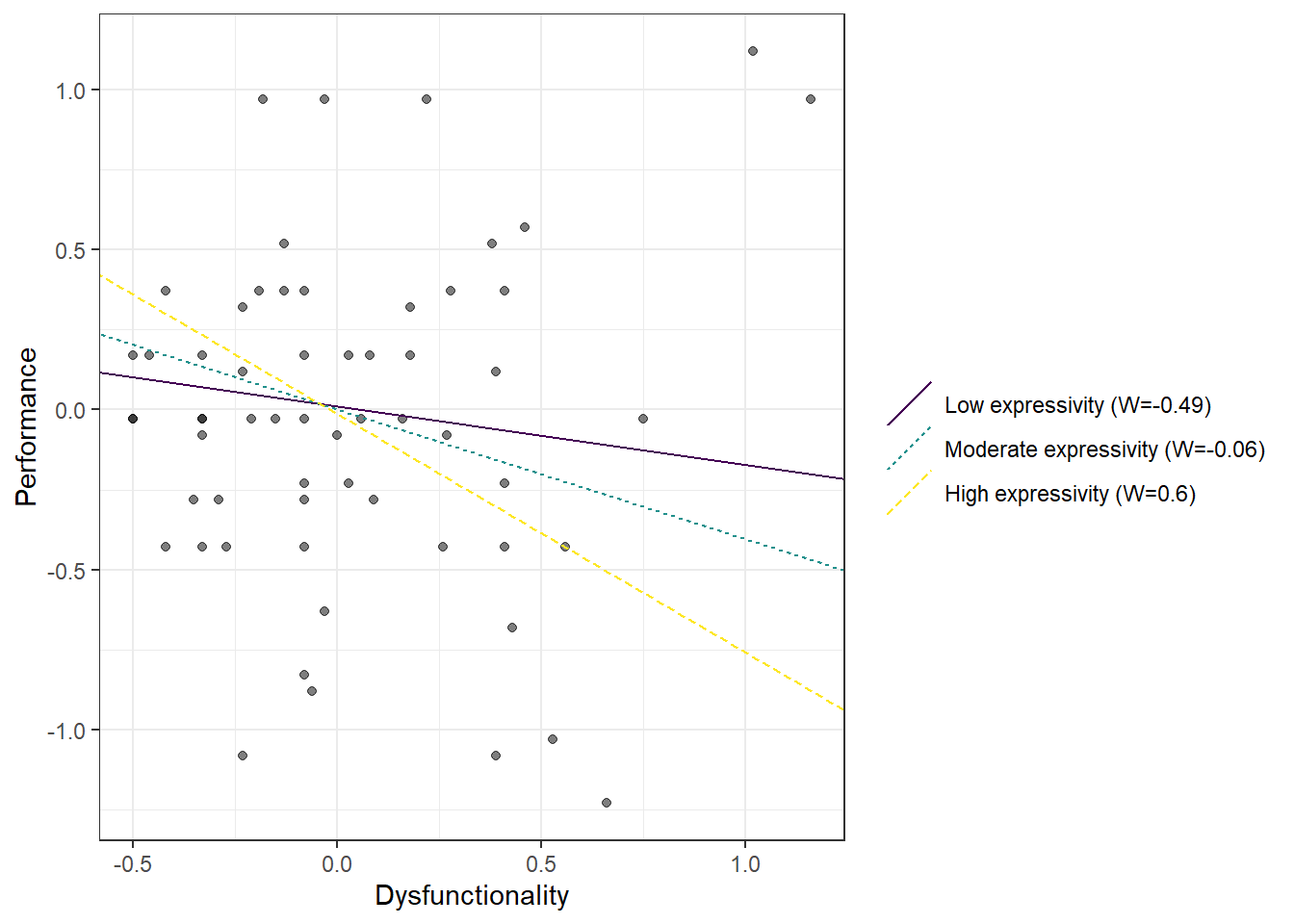

Teilaufgabe j

Von inhaltlichem Interesse ist die Größe der bedingten indirekten Effekte. Für das aktuelle Modell ergeben sich diese als das Produkt von a mit den bedingten direkten Effekten.

Konstruktion der Tabelle 11.2 (aus Hayes, 2022, S. 435) der bedingten indirekten Effekte von dysfunktionalem Teamverhalten auf die Teamleistung durch schlechtes Arbeitsklima für verschiedene Werte negativer Emotionen:

df_slope %>% mutate(a = coef(mdl_m)[2]) %>% 
             select(label, W, a, b1, b3) %>% 
             mutate(b1b3W = b1+b3*W,
                    a_b1b3W = a*b1b3W) -> tab_eff # vgl. S. 435

	W	a	b₁	b₂	b₁+b₃W	a(b₁+b₃W)
Low expressivity	-0.49	0.62	-0.436	-0.517	-0.182	-0.113
Moderate expressivity	-0.06	0.62	-0.436	-0.517	-0.405	-0.251
High expressivity	0.60	0.62	-0.436	-0.517	-0.746	-0.462

\(W\) quantifiziert den Betrag, um den sich zwei Fälle, die sich bei \(X\) um eine Einheit unterscheiden (mit einem bestimmten gegebenen Wert \(W\)), schätzungsweise bei \(Y\) indirekt durch die Wirkung von \(X\) auf \(M\) unterscheiden, was wiederum \(Y\) beeinflusst. Betrachten wir also zwei Teams, die sich bei negativen Emotionen um \(W = 0.600\) Einheiten, aber bei dysfunktionalem Verhalten um eine Einheit unterscheiden. Nach dieser Analyse (siehe Tabelle oben) ist die Leistung des Teams, das eine Einheit mehr dysfunktionales Verhalten zeigt, schätzungsweise um \(0.462\) Einheiten niedriger (weil der bedingte indirekte Effekt negativ ist), und zwar aufgrund des negativeren Arbeitsklimas, das durch das stärker dysfunktionale Verhalten erzeugt wird (weil a positiv ist), was die Teamleistung senkt (weil \(\theta_{M \rightarrow Y}\) bei \(W = 0.600\) negativ ist).

Die indirekte Auswirkung von dysfunktionalem Verhalten auf die Teamleistung durch negatives Arbeitsklima ist durchweg negativ, aber sie ist negativer bei Teams mit einer relativ höheren negativen Emotionen. Relativ mehr dysfunktionales Verhalten scheint also ein negativeres Arbeitsklima einer Gruppe zu erzeugen, das sich in einer geringeren Teamleistung niederschlägt, und zwar vor allem bei Teams mit Mitgliedern, die ihre negativen Emotionen im Team kundtun.

Teilaufgabe k

Wie wird der direkte Effekt \(c′\) der Dysfunktionalität auf Produktivität interpretiert?

Für den direkte Effekt von X auf Y wird keine Moderation angenommen, es wird folglich \(c′\) in \(Y = i_Y + c'X + b_1M + b_2W + b_3MW + e_Y\) betrachtet. Dieser Effekt gibt an, wie stark sich zwei Teams, die sich in ihrem dysfunktionalen Verhalten um eine Einheit unterscheiden, in ihrer Leistung unterscheiden, wenn Arbeitsklima und negative Emotionalität konstant bleiben. Der direkte Effekt ist positiv, \(c′ = 0.366\). Zwei Teams mit gleich negativem Arbeitsklima und gleich negativer Emotionalität, die sich aber in ihrem dysfunktionalen Verhalten um eine Einheit unterscheiden, unterscheiden sich also schätzungsweise um 0.366 Einheiten in der Teamleistung. Dabei schneidet das Team, das mehr dysfunktionales Verhalten zeigt, besser ab!

Aufgabe 2

Wiederholen Sie die Analysen mit PROCESS.

Zeichnen Sie ein konzeptuelles Diagramm der vier Variablen. Die Modellnummer ist 14.
Berechnen Sie deskriptive Kennwerte (Mittelwert und Standardabweichung).
Formulieren Sie sowohl das Modell des Mediators sowie das Modell der Produktivität.
Berechnen Sie die beiden Modellgleichungen mit zwei Regressionsmodellen.
Wie wird die Steigung des Modells für den Mediator interpretiert? Ist diese Steigung signifikant?
Ist negexp ein Moderator.
Wie werden die Steigungen von \(M\) und \(W\) interpretiert?
Anstatt die \(b_3\) Steigung direkt zu interpretieren, betrachtet man den bedingten Effekt des negativen Arbeitsklimas auf die Produktivität, der eine Funktion der Sichtbarkeit ist. Wie lautet dieser bedingte Effekt.
Um den bedingten Effekt besser zu verstehen, wird er für einen kleinen, mittleren und großen Wert des Moderators berechnet. Hayes schlägt vor, die bedingten Effekte des 16., 50. und 84. Perzentils zu verwenden. Um einen Simple-Slopes-Plot zu erhalten, kann in process den Parameter plot=1 verwendet werden. Fertigen Sie einen Simple-Slopes-Plot an.
Von inhaltlichem Interesse ist die Größe der bedingten indirekten Effekte. Für das aktuelle Modell ergeben sich diese als das Produkt von a mit den bedingten direkten Effekten.
Wie wird der direkte Effekt \(c′\) der Dysfunktionalität auf Produktivität interpretiert?

Anstelle des Macros kann processR via devtools installiert werden (install_github("cardiomoon/processR"))¹.

Teilaufgabe a

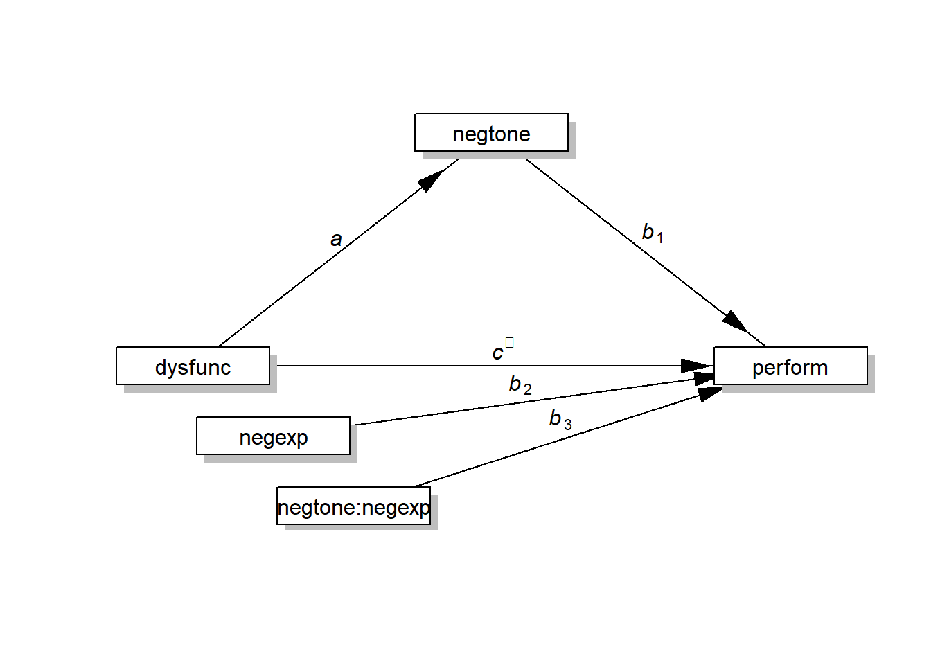
Zeichnen Sie ein konzeptuelles Diagramm der vier Variablen. Die Modellnummer ist 14.

Dies kann mit dem Befehl pmacroModel() geschehen, die Labels (X, M, Y, W) können wie folgt angepasste werden:

labels = list(X = "dysfunc", M = "negtone", Y = "perform", W = "negexp")
pmacroModel(14, labels = labels)

Teilaufgabe b

Berechnen Sie deskriptive Kennwerte (Mittelwert und Standardabweichung).

Siehe Aufgabe 1.b. (oben)

Teilaufgabe c

Formulieren Sie sowohl das Modell des Mediators sowie das Modell der Produktivität.

moderator <- list(name = "negexp", site = c("b"))
model <- tripleEquation(X = "dysfunc", M = "negtone", Y = "perform", 
                        moderator = moderator)
cat(model)

negtone~a*dysfunc
perform~c*dysfunc+b1*negtone+b2*negexp+b3*negtone:negexp
negexp ~ negexp.mean*1
negexp ~~ negexp.var*negexp
CE.MonY :=b1+b3*negexp.mean
indirect :=(a)*(b1+b3*negexp.mean)
index.mod.med :=a*b3
direct :=c
total := direct + indirect
prop.mediated := indirect / total
CE.MonY.below :=b1+b3*(negexp.mean-sqrt(negexp.var))
indirect.below :=(a)*(b1+b3*(negexp.mean-sqrt(negexp.var)))
CE.MonY.above :=b1+b3*(negexp.mean+sqrt(negexp.var))
indirect.above :=(a)*(b1+b3*(negexp.mean+sqrt(negexp.var)))
direct.below:=c
direct.above:=c
total.below := direct.below + indirect.below
total.above := direct.above + indirect.above
prop.mediated.below := indirect.below / total.below
prop.mediated.above := indirect.above / total.above

Mit dieser Modellsyntax kann die moderierte Mediation mittels sem() Funktion aus dem 📦 lavaan-Paket durchgeführt werden.

Teilaufgabe d

Berechnen Sie die beiden Modellgleichungen mit zwei Regressionsmodellen.

semfit <- sem(model = model, data = df_proc)
estimatesTable(semfit)

  Variables     Predictors label     B   SE     z       p     β
1   negtone        dysfunc     a  0.62 0.16  3.78 < 0.001  0.44
2   perform        dysfunc     c  0.37 0.17  2.19   0.029  0.27
3   perform        negtone    b1 -0.44 0.12 -3.68 < 0.001 -0.46
4   perform         negexp    b2 -0.02 0.10 -0.19   0.852 -0.02
5   perform negtone:negexp    b3 -0.52 0.20 -2.57   0.010 -0.29

# estimatesTable2(semfit)

Siehe auch summary(semfit) für eine vollständige Ausgabe der Ergenisse.

statisticalDiagram(14, labels = labels, fit = semfit, whatLabel = "est")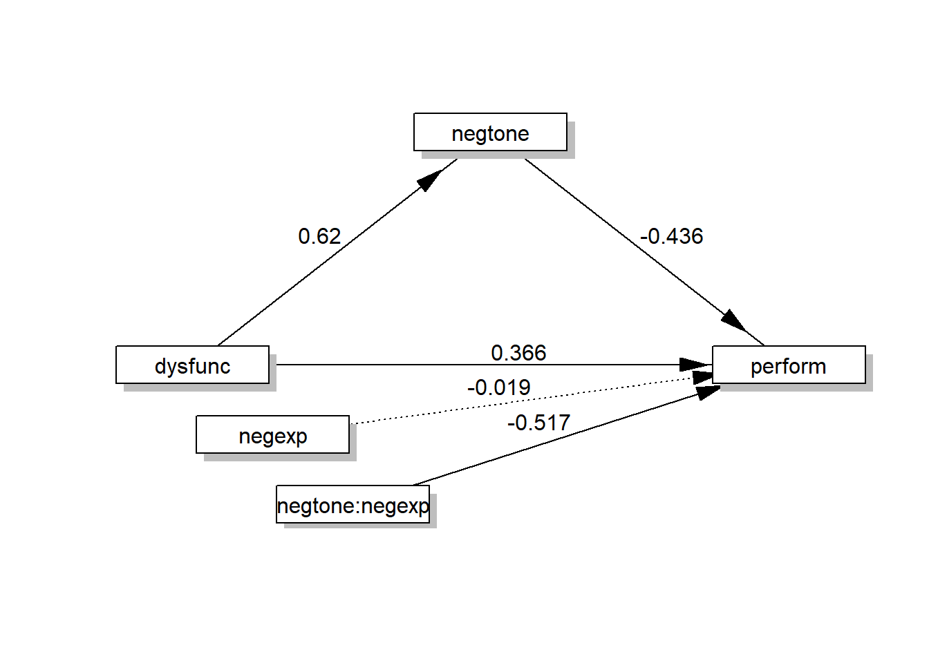

Teilaufgaben e-k

Siehe entsprechende Teilaufgaben in Aufgabe 1, die Interpretationen sind äquivalant.

Literatur

Cole, M. S., Walter, F., & Bruch, H. (2008). Affective mechanisms linking dysfunctional behavior to performance in work teams: a moderated mediation study. Journal of Applied Psychology, 93(5), 945–958. https://doi.org/10.1037/0021-9010.93.5.945

Hayes, A. F. (2022). Introduction to mediation, moderation, and conditional process analysis: A regression-based approach (3. Aufl.). Guilford Publications.

Fußnoten

es handelt sich um ein R-Paket von Keon-Woong Moon, Andrew F. Hayes war nicht an der Entwicklung dieses Pakets beteiligt, das Paket bietet jedoch diverse analoge Funktionen ↩︎