Einführung

Sich mit Matrizen auseinanderzusetzen ist von großer Bedeutung, da sie in der Multivariaten Statistik sehr häufig verwendet werden. Wie in den bisherigen Posts deutlich wurde, ist es zwar auch möglich, den Einsatz von Matrizen zu umgehen¹, jedoch bieten ihr Einsatz zahlreiche Vorteile, wie die bessere Lesbarkeit von Gleichungen oder die Möglichkeit, mehrere lineare Gleichungen zu einer Gleichung (in Matrizenschreibweise) zusammenzufassen. Dies soll am Beispiel der multiplen linearen Regression verdeutlicht werden:

Die Gleichung einer einzelnen Beobachtung, welche die abhängige Variable mit $\small k$ Prädiktoren vorhersagt lautet: $\small \hat{y}=b_0+b_1x_1+b_2+x_2+\cdots+b_kx_k$, in Matrixschreibweise schreibt man: $\small \hat{y}=\mathbf{x'b}$
die Gleichungen einer Stichproben des Umfangs $\small n$, welche die abhängige Variable mit $\small k$ Prädiktoren vorhersagt, werden in Matrixschreibweise zu folgender Gleichung zusammengefasst: $\small \mathbf{\hat{y}}=\mathbf{X'b}$
die Kleinste-Quadrate Methode zur Ermittlung der Regressionskoeffizienten, führt zur Lösung eines Gleichungssystems, welches mit Matrizen folgendermaßen lautet $\small \mathbf{(X'X)b}=\mathbf{X'y}$

Terminologie

Eine Matrix ist eine rechteckige Anordnung von Zahlen in mehreren Zeilen und Spalten

die Anzahl der Zeilen und Spalten entsprechen den Abmessungen der Matrix
eine $\small n\times m$–Matrix hat $\small n$ Zeilen und $\small m$ Spalten
die einzelnen Werte einer Matrix werden Elemente der Matrix genannt
ein Element der Matrix $\small \mathbf{A}$² wird als $a_{ij}$ bezeichnet
der erste Index gibt die Zeile und der zweite die Spalte an, in welcher das Element steht
ein Element kann sich folglich
- in einer Zeile an Postion $\small i=1, \dots, n$ bzw.
- in einer Spalte an Postion $\small j=1, \dots, m$ befinden
eine $\small 3\times 4$-Matrix kann allgemein geschrieben werden (links) bzw. mit Zahlenwerten (exemplarisch rechts); für das Beispiel ist exemplarisch für das Element $\small a_{21}=8$

\[ \small \mathbf{A}=\begin{pmatrix} a_{11} & a_{12} & a_{13} & a_{14} \\ a_{21} & a_{22} & a_{23} & a_{24} \\ a_{31} & a_{32} & a_{33} & a_{34} \end{pmatrix},~~ \mathbf{A}=\begin{pmatrix} 0 & 1 & 5 & 7 \\ 8 & 5 & 4 & 3 \\ 8 & 1 & 7 & 3 \end{pmatrix} \]

Gleichheit: Zwei $\small n\times m$-Matrizen $\small \mathbf{A}$ und $\small \mathbf{B}$ sind genau dann gleich, wenn jedes Element der einen Matrix dem korrespondierenden Element der anderen Matrix entspricht (d.h. ungleich, wenn sich wenigstens ein korrespondierendes Element unterscheidet)
für die tiefere Terminologie kann untergliedert werden in
- die Bezeichnung besonderer Matrizen (Zeilenvektor, Spaltenvektor, Skalar, quadratische Matrix, symmetrische Matrix, Einheitsmatrix, Diagonalmatrix, …)
- die Umformung einer Matrix (Transponierte Matrix, Inverse Matrix,…)
- die Berechnungen mit Matrizen (Addition von Matrizen, Multiplikation von Matrizen, Skalarmultiplikation, …)
- die Rechengesetze (Assoziativgesetz, Distributivgesetz, Kommutativgesetz)

Spezielle Formen

Vektor ($\small n\times 1$- bzw. $\small 1\times n$-Matrix)

Eine Matrix, die nur aus einer Spalte oder Zeile besteht, heißt Vektor
Beispiel
- für einen Spaltenvektors $\small \mathbf{v}$³ mit $\small n$ Elementen (aka. eines $\small 1\times n$-Vektors) ist $\small \mathbf{v}=\begin{pmatrix}v_1\\v_2\\\vdots\\v_n\end{pmatrix}$
- für einen Zeilenvektor $\small \mathbf{v'}$ mit $\small n$ Elementen (aka. eines $\small n\times 1$-Vektors) ist $\small \mathbf{v'}=\begin{pmatrix}v_1~~~v_2~~\dots~~v_n\end{pmatrix}=\begin{pmatrix}v_1,v_2,\dots, v_n\end{pmatrix}$
in der hießigen Konvention nehmen wir an, dass es sich bei allen Vektoren um Spaltenvektoren handelt (die sich jedoch in Zeilenvektoren umformen lassen, siehe Transponierte Vektoren)

Skalar ($\small 1\times 1$-Matrix)

Einen einzelnen Wert bezeichnet man im Rahmen der Matrixalgebra als Skalar
ein Skalar ist also eine reelle Zahl
Beispiele für Skalare sind $\small 0$, $\small 8$, $\small 15$ oder $\small k$⁴.

Quadratische Matrix

Eine Matrix ist quadratisch, wenn sie genauso viele Zeilen wie Spalten hat

Symmetrische Matrix

Eine quadratische Matrix heißt symmetrisch, wenn für die Elemente der Matrix $\small\mathbf{A}$ gilt: $\small a_{ij}=a_{ji}$
Beispiel einer symmetrischen Matrix: $\small \mathbf{A}=\begin{pmatrix}1 & 4 & 5\\ 4 & 2 & 6\\ 5&6&3\end{pmatrix}$

Korrelationsmatrix

Eine Korrelationsmatrix $\small\mathbf{R}$ ist symmetrisch:

\[ \small \mathbf{R}=\begin{pmatrix} 1 & r_{12} & r_{13} & \dots & r_{1p} \\ r_{21} & 1 & r_{23} & \dots & r_{2p} \\ r_{31} & r_{32} & 1 & \dots & r_{3p} \\ \vdots & \vdots & \vdots & \ddots & \vdots \\ r_{p1} & r_{p2} & r_{p3} & \dots & 1 \end{pmatrix} \]

Diagonalmatrix

Befinden sich in einer quadratischen Matrix außerhalb der Hauptdiagonale nur Nullen, so sprechen wir von einer Diagonalmatrix .

\[ \small \mathbf{D}=\begin{pmatrix} d_1 & 0 & 0 & \dots & 0 \\ 0 & d_2 & 0 & \dots & 0 \\ 0 & 0 & d_3 & \dots & 0 \\ \vdots & \vdots & \vdots & \ddots & \vdots \\ 0 & 0 & 0 &\dots & d_n \end{pmatrix} \]

Einheitsmatrix

Eine Diagonalmatrix heißt Einheitsmatrix, wenn alle Diagonalelemente den Wert 1 haben.

\[ \small \mathbf{I}=\begin{pmatrix} 1 & 0 & 0 & \dots & 0 \\ 0 & 1 & 0 & \dots & 0 \\ 0 & 0 & 1 & \dots & 0 \\ \vdots & \vdots & \vdots & \ddots & \vdots \\ 0 & 0 & 0 &\dots & 1 \end{pmatrix} \]

Die Einheitsmatrix wird mit $\mathbf{I}$ bezeichnet⁵. Ihre Abmessungen ergeben sich aus dem jeweiligen Kontext.

Nullmatrix

Eine Matrix, die nur aus Nullen besteht wird Nullmatrix genannt. Sie wird mit bezeichnet, ihre Abmessungen ergeben sich aus dem jeweiligen Kontext.

\[ \small \mathbf{0}=\begin{pmatrix} 0 & 0 & 0 & \dots & 0 \\ 0 & 0 & 0 & \dots & 0 \\ 0 & 0 & 0 & \dots & 0 \\ \vdots & \vdots & \vdots & \ddots & \vdots \\ 0 & 0 & 0 &\dots & 0 \end{pmatrix} \]

Umgeformte Matrizen

Transponierte Matrix

Eine transponierte Matrix erhalten wir, indem Zeilen mit Spalten “vertauscht” werden.

Die Transponierte einer Matrix $\small\mathbf{A}$ wird mit $\small\mathbf{A'}$ (oder $\small\mathbf{A^T}$) gekennzeichnet.
Wird beispielsweise $\small \mathbf{A}=\begin{pmatrix}3&1&2 \\ 5&0&4 \end{pmatrix}$ transponiert, ergibt sich $\small \mathbf{A'}=\begin{pmatrix}3&5\\ 1&0 \\ 2&4\end{pmatrix}$
Die Transposition einer transponierten Matrix ergibt wieder die ursprüngliche Matrix: $\small(\mathbf{A'})'=\mathbf{A}$
Für symmetrische Matrizen gilt: $\small\mathbf{A'}=\mathbf{A}$

Transponierte Vektoren

Oft wird vereinbart: Alle Vektoren sind Spaltenvektoren.
Somit ist ein Zeilenvektor ein transponierter Spaltenvektor und es gilt:
- Der Vektor $\small\mathbf{v}$ steht in einer Spalte
- Der Vekto $\small\mathbf{v'}$ steht in einer Zeile
Notation: $\small \mathbf{v}=\begin{pmatrix}v_1\\ v_2\\\vdots\\v_n \end{pmatrix}$ und $\small \mathbf{v}=\begin{pmatrix}v_1, v_2, \dots, v_n \end{pmatrix}$

Inverse Matrix

die Inverse einer regulären Matrix ist im Allgemeinen schwer zu bestimmen
für eine reguläre $\small 2\times 2$-Matrix gibt es eine einfache Formel für die Inverse
sei $\small \mathbf{A}=\begin{pmatrix}a & b\\c & d \end{pmatrix}$ regulär, dann lautet die Inverse:

\[ \small \mathbf{A}^{-1}=\frac{1}{\mid A\mid}\begin{pmatrix}~~~d & -b\\-c & ~~~a \end{pmatrix} =\frac{1}{ad-bc}\begin{pmatrix}~~~d & -b\\-c & ~~~a \end{pmatrix} \]

Rechnen mit Matrizen

Skalarmultiplikation

Eine Matrix darf mit einem Skalar multipliziert werden.
Bezeichnen wir das Skalar mit $\small k$und die $\small (n\times n)$-Matrix mit $\small \mathbf{A}$, so schreiben wir die Skalarmultiplikation als $\small k\mathbf{A}$.
Beispiel: Sei $\small \mathbf{A}$ die Matrix $\small \mathbf{A}=\begin{pmatrix}3&1&2 \\ 1&2&4 \end{pmatrix}$ und $\small k=2$, dann ergibt sich durch Skalarmultiplikation $\small k\mathbf{A}$ die Matrix $\small k\mathbf{A}=\begin{pmatrix}6&2&4 \\ 2&4&8 \end{pmatrix}$

Matrixaddition

Um zwei Matrizen addieren zu können, müssen sie die gleiche Anzahl von Zeilen und Spalten aufweisen
Matrizen werden addiert, indem jedes Element der Summe gleich der Summe der korrespondierenden Elemente der addierten Matrizen ist
für $\small \mathbf{A+B}$ ergeben sich die Elemente als $\small a_{ij}+b_{ij}=c_{ij}$ für $\small i=1, \dots,n$ und $\small j=1, \dots,m$
Beispiel:
- Gegeben seien die Matrizen $\small \mathbf{A}=\begin{pmatrix}3 & 1\\5 & 2\\2&4 \end{pmatrix}$ und $\small \mathbf{B}=\begin{pmatrix}5 & 4\\1 & 2\\1 & 3\end{pmatrix}$
- die Summenmatrix $\small \mathbf{A+B} = \mathbf{C}$ ergibt sich durch die Berechnung:
\[\small \mathbf{A+B} = \begin{pmatrix}3 & 1\\5 & 2\\2&4 \end{pmatrix} + \begin{pmatrix}5 & 4\\1 & 2\\1 & 3\end{pmatrix} = \begin{pmatrix}8 & 5\\6 & 4\\3 & 7\end{pmatrix} = \mathbf{C}\]

Matrixmultiplikation

Die Multiplikation zweier Matrizen ist nur möglich, wenn die Anzahl der Spalten der linken Matrix gleich der Zeilenanzahl der rechten Matrix ist
wir nehmen deshalb an, dass $\small \mathbf{A}$ eine $\small n\times s$-Matrix und $\small \mathbf{B}$ eine $\small s\times m$-Matrix ist
die Multiplikation $\small \mathbf{AB}$ führt zu einer Matrix $\small \mathbf{C}$ mit der Ordnung $\small n\times m$
die Matrizenmultiplikation erfolgt nach der Regel $\small c_{ij}=\sum_{k=1}^s a_{ik}b_{kj}$, für $\small i=1, \dots,n$ und $\small j=1, \dots,m$
Beispiel:
- Gegeben seien die Matrizen $\small \mathbf{A}=\underbrace{\begin{pmatrix}3 & 1 & 2\\5 & 2 & 2\end{pmatrix}}_{2\times 3}$ und $\small \mathbf{B}=\underbrace{\begin{pmatrix}5 & 4\\1 & 2\\1 & 3\end{pmatrix}}_{3\times 2}$
- weil $\small s=2$ (3 Spalten in $\small \mathbf{A}$ und 3 Zeilen in $\small \mathbf{B}$) ist die Multiplikation $\small \mathbf{AB}$ möglich
- die aus $\small \mathbf{AB}$ resultierende Matrix $\small \mathbf{C=AB}$ ist eine $\small 2\times 2$-Matrix (weil $\small \mathbf{A} n = 2$ Zeilen und $\small \mathbf{B} m = 2$ Spalten hat)
- für die exemplarische Berechnung s.u.
- man erhält $\small \mathbf{C}=\begin{pmatrix}3 & 1 & 2\\5 & 2 & 2\end{pmatrix}\begin{pmatrix}5 & 4\\1 & 2\\1 & 3\end{pmatrix}=\begin{pmatrix}18 & 20\\29 & 30\end{pmatrix}$
- die aus $\small \mathbf{BA}$ resultierende Matrix $\small \mathbf{D=BA}$ ist hingehen eine $\small 3\times 3$-Matrix
- man erhält $\small \mathbf{D}=\begin{pmatrix}5 & 4\\1 & 2\\1 & 3\end{pmatrix}\begin{pmatrix}3 & 1 & 2\\5 & 2 & 2\end{pmatrix}=\begin{pmatrix}35 & 13 & 18\\13 & 5 & 6 \\ 18 & 7 & 8\end{pmatrix}$

Beispielrechnung C

\[ \small \begin{align*} \mathbf{AB} & = \begin{pmatrix}3 & 1 & 2\\5 & 2 & 2\end{pmatrix}\begin{pmatrix}5 & 4\\1 & 2\\1 & 3\end{pmatrix}\\ & = \begin{pmatrix}[3\cdot 5 + 1\cdot 1 + 2\cdot 1] & [3\cdot 4 + 1\cdot 2 + 2\cdot 3] \\ [5\cdot 5 + 2\cdot 1 + 2\cdot 1] & [5\cdot 4 + 2\cdot 2 + 2\cdot 3]\end{pmatrix}\\ & =\begin{pmatrix}[15+1+2] & [12+2+6] \\ [25+2+2] & [20+4+6]\end{pmatrix}\\ & = \begin{pmatrix}18 & 20\\29 & 30\end{pmatrix} = \mathbf{C} \end{align*} \]

Inneres und äußeres Produkt von Vektoren

Werden zwei Vektoren miteinander multipliziert, unterscheidet man zwischen einem inneren Produkt und einem äußeren Produkt
- inneres Produkt: $\small \mathbf{u'v}$
- äußeres Produkt: $\small \mathbf{uv'}$
das innere Produkt wird auch Skalarprodukt genannt
Achtung: Man verwechsle nicht das Skalarprodukt mit der Skalarmultiplikation
Beispiele:
- Geben seien die Vektoren $\small \mathbf{u'}= \begin{pmatrix}1 & 2 & 3\end{pmatrix}$ und $\small \mathbf{v'}= \begin{pmatrix}4 & 5 & 6\end{pmatrix}$
- dann ergibt sich für das innere Produkt $\small \mathbf{u'v}$ ein Skalar $\small \mathbf{u'v}= \begin{pmatrix}1 & 2 & 3\end{pmatrix}\begin{pmatrix}4 \\ 5 \\ 6\end{pmatrix}=1\cdot4 + 2\cdot 5 + 3\cdot 6 = 32$
- für das äußere Produkt $\small \mathbf{uv'}$ ergibt sich die Matrix $\small \mathbf{uv'}= \begin{pmatrix}1\\2\\3\end{pmatrix}\begin{pmatrix}4&5&6\end{pmatrix}=\begin{pmatrix}4&5&6\\8&10&12\\12&15&18\end{pmatrix}$

Transponieren eines Produkts

Ferner gilt, dass die Transponierte eines Matrizenprodukts gleich dem Produkt der transponierten Matrizen in umgekehrter Reihenfolge ist:

\[\small \mathbf{(AB)'}=\mathbf{B'A'}\]

Neutrales und inverses Element

Matrizen, die eine Inverse besitzen, werden regulär genannt
Matrizen, die keine Inverse besitzen, werden singulär genannt
Beispiel:
- die folgende Matrix $\small \mathbf{A} = \begin{pmatrix}1 & 1 \\ 0 & 2\end{pmatrix}$ besitzt eine Inverse
- ihre Inverse ist $\small \mathbf{A}^{-1} = \begin{pmatrix}1 & -0.5 \\ 0 & ~~~0.5\end{pmatrix}$
- folglich ist $\small \mathbf{A}$ regulär

Addition

Die Nullmatrix ist das neutrale Element der Addition. Also: $\small \mathbf{A+0=A}$ Das inverse Element der Addition lautet $\small \mathbf{-A}$. Also: $\small \mathbf{A-A=0}$

Multiplikation

Multiplikationen mit der Einheitsmatrix $\small \mathbf{I}$ verändern die Matrix $\small \mathbf{A}$ nicht: $\small \mathbf{AI=IA=A}$

Die Einheitsmatrix $\small \mathbf{I}$ ist also das neutrale Element der Multiplikation
ein inverses Element der Matrizenmultiplikation existiert nicht immer
eine notwendige Voraussetzung für die Existenz der Inversen ist, dass die Matrix quadratisch ist
falls die zu $\small \mathbf{A}$ inverse Matrix existiert, wird sie mit $\small \mathbf{A}^{-1}$ bezeichnet
in diesem Fall gilt: $\small \mathbf{AA}^{-1}=\mathbf{A}^{-1}\mathbf{A}=\mathbf{I}$

Determinante

Für eine quadratische Matrix kann die sog. Determinante berechnet werden
die Determinante einer Matrix ist eine reelle Zahl
eine Determinante wird durch zwei senkrechte Striche gekennzeichnet, d.h. die Determinante von $\small \mathbf{A}$ wird mit $\small \mathbf{|A|}$ bezeichnet
ist die Determinante einer Matrix ist genau dann von null verschieden, wenn die Matrix regulär ist, d.h. eine Inverse besitzt
der Aufwand zur Berechnung der Determinante steigt mit der Dimension der Matrix schnell an, sodass eine Formel nur für den Fall einer $\small 2\times 2$ Matrix gegeben wird
für die Matrix $\small \mathbf{A} = \begin{pmatrix}a_{11} & a_{12} \\ a_{21} & a_{22}\end{pmatrix}$ berechnet man die Determinante $\small \mathbf{|A|}$ als $\small \mathbf{|A|}= a_{11}a_{22}-a_{12}a_{21}$
Beispiele:
- sei $\small \mathbf{A} = \begin{pmatrix} 1 & 1 \\ 0 & 2\end{pmatrix}$, dann lautet die Determinante: $\small \mathbf{|A|}= a_{11}a_{22}-a_{12}a_{21} = 1\cdot2 - 1\cdot0 = 2$. Also ist $\small \mathbf{A}$ regulär (kann invertiert werden)
- sei $\small \mathbf{A} = \begin{pmatrix} 2 & 4 \\ 5 & 10\end{pmatrix}$, dann lautet die Determinante: $\small \mathbf{|A|}= 2\cdot10 - 5\cdot4 = 0$. Also ist $\small \mathbf{A}$ singulär (kann nicht invertiert werden)

Gesetzmäßigkeiten

Kommutativgesetz

Die Addition zweier Matrizen ist kommutativ, d. h. die Reihenfolge der Summanden ist beliebig. Es gilt somit:

\[\small \mathbf{A+B} = \mathbf{B+A} \]

Die Multiplikation zweier Matrizen ist nicht kommutativ, d. h. im allgemeinen gilt:

\[\small \mathbf{AB} \neq \mathbf{BA} \]

Assoziativgesetz

Die Addition ist assoziativ:

\[\small \mathbf{(A+B)+C} = \mathbf{A+(B+C)}= \mathbf{A+B+C} \]

Die Multiplikation ist assoziativ:

\[\small \mathbf{(AB)C} = \mathbf{A(BC)}= \mathbf{ABC} \]

Distributivgesetz

\[ \small \begin{align*} \mathbf{(A+B)C} & = \mathbf{AC+BC}\\ \mathbf{A(B+C)} & = \mathbf{AB+AC} \end{align*} \]

weitere Eigenschaften von Matrizen

Lineare Abhängigkeit

Zwei Vektoren $\small \mathbf{a_1}$ und $\small \mathbf{a_2}$ sind linear abhängig, falls es reelle Koeffizienten $\small c_1$ und $\small c_2$ gibt, die nicht alle null sind, und für die $\small c_1\mathbf{a_1}+c_2\mathbf{a_2}=\mathbf{0}$ erfüllt ist
mit anderen Worten, falls die Gleichung nur für $c_1=c_2=0$ erfüllt ist, sind die Vektoren linear unabhängig
für mehr als zwei Vektoren lässt sich die lineare Abhängigkeit ganz analog erklären
Beispiel:
- sind die Vektoren $\small \mathbf{a_1}=\begin{pmatrix} 2 \\ 5 \end{pmatrix}$ und $\small \mathbf{a_2}=\begin{pmatrix} 4 \\ 10 \end{pmatrix}$ linear abhängig?
- ja, denn für $\small c_1=2$ und $\small c_2=-1$ 1ergibt sich der Nullvektor: $\small 2\cdot\begin{pmatrix} 2 \\ 5 \end{pmatrix}-1\cdot\begin{pmatrix} 4 \\ 10 \end{pmatrix}=\begin{pmatrix} 4 \\ 10 \end{pmatrix}-\begin{pmatrix} 4 \\ 10 \end{pmatrix}=\mathbf{0}$

Determinanten und lineare Abhängigkeit

eine Matrix kann als aus Vektoren bestehend betrachtet werden
die Matrix $\small \mathbf{A}=\begin{pmatrix} a_{11}&a_{12} \\ a_{21}&a_{22} \end{pmatrix}$ kann als $\small\begin{pmatrix} \mathbf{a_1}&\mathbf{a_2} \end{pmatrix}$ geschrieben werden, wobei $\small \mathbf{a_1}=\begin{pmatrix} a_{11} \\ a_{21} \end{pmatrix}$ und $\small \mathbf{a_2}=\begin{pmatrix} a_{12} \\ a_{22} \end{pmatrix}$
eine Determinante von null resultiert, wenn die Spalten der Matrix, d.h. $\small \mathbf{a_1}$ und $\small \mathbf{a_2}$ lineare abhängig sind
Beispiel:
- Die Matrix $\small \mathbf{A}=\begin{pmatrix} 2&4 \\ 5&10 \end{pmatrix}$ besitzt eine Determinante von null, weil ihre Spalten linear abhängig sind

Rang einer Matrix

Der Spaltenrang einer Matrix ist die Anzahl der linear unabhängigen Spalten.
der Zeilenrang einer Matrix ist die Anzahl der linear unabhängigen Zeilen.
für jede Matrix gilt: Zeilenrang = Spaltenrang.
entspricht der Rang einer quadratischen Matrix der Anzahl ihrer Spalten (Zeilen), dann hat sie vollen Rang
Matrizen mit vollem Rang sind regulär, d.h. besitzen eine Inverse
Beispiel:
- Wie lautet der Rang folgender Matrix $\small \mathbf{A} = \begin{pmatrix}1 & 1 & 0 & 0\\ 1 & 0 & 1 & 0 \\ 1 & 0 & 0 & 1\end{pmatrix}$
- Da die erste Spalte gleich der Summe der letzten drei Spalten ist, sind die vier Spalten linear abhängig
- offensichtlich sind die letzten drei Spalten aber linear unabhängig
- Somit ist der Rang der Matrix 3

R/SPSS

R-Pakete

Es werden keine Pakete benötigt, sämtliche Funktionen sind Teil von base-R. In SPSS erfolgt die Berechnung ebenfalls syntaxgebunden.

Base-R und SPSS Syntax

Es wird mit der folgenden Matrix $\small\mathbf{M}$ exemplarisch gerechnet:

\[ \small \mathbf{M}=\begin{pmatrix} 1 & 2 & 3\\ 3 & 2 & 1 \end{pmatrix} \]

R
SPSS

Eine Matrix $\small \mathbf{M}$ kann in R mit dem Befehl matrix() erstellt werden. Das Argument byrow ist dabei per default auf FALSE gesetzt!

M <- matrix(data = c(1, 2, 3, 3, 2, 1),
            byrow = TRUE,
            ncol = 3)
M

     [,1] [,2] [,3]
[1,]    1    2    3
[2,]    3    2    1

In SPSS müssen sämtliche Matrix-Operationen in einer entsprechenden Matrix-Umgebung durchgeführt werden. Eine Matrix $\small \mathbf{M}$ wird durch COMPUTE initial erzeugt und hier in der Variable M abgespeichert. Die Elemente werden in geschweifte Klammern geschrieben, wie in R durch Kommata geterennt, allerdings zeilenweise, wobei mit ; in eine neue Zeile gewechselt wird:

MATRIX

COMPUTE M = {1, 2, 3; 3, 2, 1}.
PRINT M.

END MATRIX.

Anmerkung. Die nachfolgenden Funktionen funktionieren selbstverständlich nur für passende Matrizen für welche M ein Platzhalter ist (es ist also nicht zwangsläufig die Beispielmatrix $\small \mathbf{M}$ von oben gemeint).

Funktion	R	SPSS
Transponieren	`t(M)`	`T(M)`
Determinante	`det(M)`	`DET(M)`
Invertieren	`solve(M)`	`INV(M)`
Rang	`qr(M)$rank`	`RANK(M)`

Für eiene Anwandung siehe die folgenden Übungsaufgaben.

Übungsaufgaben

Aufgabe 1

Gegeben sind die Matrizen $\small \mathbf{A}$ und $\small \mathbf{B}$:

\[ \small \mathbf{A}=\begin{pmatrix} 1 & 2 & 3\\ 3 & 2 & 1 \end{pmatrix},~~ \mathbf{B}=\begin{pmatrix} 4 & -2 & 0\\ 6 & 2 & 1 \end{pmatrix} \]

Berechnen Sie die folgenden Ausdrücke: $\small \mathbf{A}+\mathbf{B}$, $\small 2\mathbf{A}$ und $\small \mathbf{B}-\mathbf{A}$.
Welche der Matrixprodukte $\small \mathbf{AB}$, $\small \mathbf{BA}$, $\small \mathbf{BA'}$ und $\small \mathbf{AB'}$ sind erklärt? Welche Abmessungen haben die resultierenden Matrizen? Berechnen Sie die Produkte, die erklärt sind.
Die beiden Matrizen $\small \mathbf{BA'}$ und $\small \mathbf{AB'}$ sind eng verwandt. In welcher Weise und auf welche Regel weist dies hin?

R
SPSS

A <- matrix(data = c(1, 2, 3, 
                     3, 2, 1), 
            ncol = 3, byrow = TRUE)

B <- matrix(data = c(4, -2, 0, 
                     6,  2, 1), 
            ncol = 3, byrow = TRUE)
A; B

     [,1] [,2] [,3]
[1,]    1    2    3
[2,]    3    2    1

     [,1] [,2] [,3]
[1,]    4   -2    0
[2,]    6    2    1

MATRIX   
  
COMPUTE A = {1, 2, 3; 3, 2, 1}.
COMPUTE B = {4, -2, 0; 6, 2, 1}.


END MATRIX.

Teilaufgabe a

Berechnen Sie die folgenden Ausdrücke: $\small \mathbf{A}+\mathbf{B}$, $\small 2\mathbf{A}$ und $\small \mathbf{B}-\mathbf{A}$.

Addition von Matrizen

Es wird die Summe eines jeden Elements der Position $\small i,j$ einer Matrix ($\small \mathbf{A}$) dem korreskondierenden Element der zu addierenden Matrix gebildet. Dies ist nur möglich, wenn beide Matrizen dieselben Ausmaße haben (hier gegeben, beide $\small 2\times3$). Auch die reulultierende Matrix hat dann diese Dimensionen inne:

\[ \small \begin{align*} \mathbf{A}+\mathbf{B}&=\underbrace{\begin{pmatrix} 1 & 2 & 3\\ 3 & 2 & 1 \end{pmatrix}}_{2\times3}+ \underbrace{\begin{pmatrix} 4 & -2 & 0\\ 6 & 2 & 1 \end{pmatrix}}_{2\times3}\\ &=\begin{pmatrix} 1+4 & 2-2 & 3+0\\ 3+6 & 2+2 & 1+1 \end{pmatrix}\\ &=\begin{pmatrix} 5 & 0 & 3\\ 9 & 4 & 2 \end{pmatrix} \end{align*} \]

R
SPSS

A+B

     [,1] [,2] [,3]
[1,]    5    0    3
[2,]    9    4    2

MATRIX   
  
COMPUTE C = A+B.
PRINT C.

END MATRIX.

Multiplikation mit einem Skalar

Jedes Element einer Matrix ($\small \mathbf{A}$) wird mit dem Skalar (2) multipliziert. Es resultiert eine Matrix derselben Dimensionen wie der Ursprungsmatrix:

\[ \small \begin{align*} 2\cdot\mathbf{A} &= 2\cdot \begin{pmatrix} 1 & 2 & 3\\ 3 & 2 & 1 \end{pmatrix}\\ &= \begin{pmatrix} 2\cdot1 & 2\cdot2 & 2\cdot3\\ 2\cdot3 & 2\cdot2 & 2\cdot1 \end{pmatrix}\\ &= \begin{pmatrix} 2 & 4 & 6\\ 6 & 4 & 2 \end{pmatrix} \end{align*} \]

R
SPSS

2*A

     [,1] [,2] [,3]
[1,]    2    4    6
[2,]    6    4    2

MATRIX   
  
COMPUTE k=2.
COMPUTE C = k*A.
PRINT C.

END MATRIX.

Subtraktion von Matrizen

Die Subtraktion von Matrizen folgt den jegeln und der Voraussetzung der Addition von Matrizen, wobei subtrahiert statt addiert wird:

\[ \small \begin{align*} \mathbf{A}-\mathbf{B}&=\begin{pmatrix} 1 & 2 & 3\\ 3 & 2 & 1 \end{pmatrix} \begin{pmatrix} 4 & -2 & 0\\ 6 & 2 & 1 \end{pmatrix}\\ &=\begin{pmatrix} 1-4 & 2+2 & 3-0\\ 3-6 & 2-2 & 1-1 \end{pmatrix}\\ &=\begin{pmatrix} -3 & 4 & 3\\ -3 & 0 & 0 \end{pmatrix} \end{align*} \]

R
SPSS

B-A

     [,1] [,2] [,3]
[1,]    3   -4   -3
[2,]    3    0    0

MATRIX   
  
COMPUTE C = B-A.
PRINT C.

END MATRIX.

Teilaufgabe b

Welche der Matrixprodukte $\small \mathbf{AB}$, $\small \mathbf{BA}$, $\small \mathbf{BA'}$ und $\small \mathbf{AB'}$ sind erklärt? Welche Abmessungen haben die resultierenden Matrizen? Berechnen Sie die Produkte, die erklärt sind.

Multiplikation von Matrizen

Für die Multiplikation von Matrizen bedarf es bestimmter Abmessungen

Es sind

\[ \small \mathbf{A'}=\begin{pmatrix} ~~1 & 3 ~~ \\ ~~2 & 2 ~~ \\ ~~3 & 1 ~~ \end{pmatrix},~~ \mathbf{B'}=\begin{pmatrix} ~~~4 & 6~~ \\ -2 & 2~~ \\ ~~~0 & 1~~ \end{pmatrix} \]

Für $\mathbf{B\cdot A'}$ ergibt sich

\[ \small \begin{align*} \mathbf{B\cdot A'} & = \overbrace{\begin{pmatrix} 4 & -2 & 0\\ 6 & 2 & 1 \end{pmatrix}}^{2\times3}\cdot \overbrace{\begin{pmatrix} 1 & 3 \\ 2 & 2 \\ 3 & 1 \end{pmatrix}}^{3\times2}\\ & = \begin{pmatrix} [4\cdot1+(-2\cdot2)+0\cdot3] & [4\cdot3 + (-2\cdot2)+0\cdot1] \\ [6\cdot1+2\cdot2+1\cdot3] & [6\cdot3+2\cdot2+1\cdot1] \end{pmatrix}\\ & = \begin{pmatrix} [4-4+0] & [12-4+0] \\ [6+4+3] & [18+4+1] \end{pmatrix}\\ & = \begin{pmatrix} 0 & 8 \\ 13 & 23 \end{pmatrix} \end{align*} \]

Analog lässt sich $\mathbf{A\cdot B'}$ berechnen:

\[ \small \begin{align*} \mathbf{A\cdot B'} & = \overbrace{\begin{pmatrix} 1 & 2 & 3\\ 3 & 2 & 1 \end{pmatrix}}^{2\times3}\cdot \overbrace{\begin{pmatrix} 4 & 6 \\ -2 & 2 \\ 0 & 1 \end{pmatrix}}^{3\times2}\\ & = \begin{pmatrix} [4-4+0] & [6+4+3] \\ [12-4+0] & [18+4+1] \end{pmatrix}\\ & = \begin{pmatrix} 0 & 13 \\ 8 & 23 \end{pmatrix} \end{align*} \]

R
SPSS

Mit * können Matrizen elementenweise multipliziert werden (d. h. jene Operation, wie wir sie von der Multiplikation oder Subtraktion kennen, sprich aus A*B resultiert eine Matrix derselben Dimensionen). Sollen hingegen Matrizen als solche multipliziert werden, muss %*% als Operator genutzt werden. Die Multiplikation von Matrizen falscher Abmessung führt in beiden Fällen zu einer Fehlermeldung (d. h. weder At*B noch A%*%B liefert ein Ergebnis).

At <- t(A)
Bt <- t(B)

B %*% At

     [,1] [,2]
[1,]    0    8
[2,]   13   23

A %*% Bt

     [,1] [,2]
[1,]    0   13
[2,]    8   23

Merke. Die Position spielt eine Rolle!

At %*% B

     [,1] [,2] [,3]
[1,]   22    4    3
[2,]   20    0    2
[3,]   18   -4    1

Bt %*% A

     [,1] [,2] [,3]
[1,]   22   20   18
[2,]    4    0   -4
[3,]    3    2    1

MATRIX   
  
COMPUTE C_1 = B*T(A).
PRINT C_1.

COMPUTE C_2 = A*T(B).
PRINT C_2.

END MATRIX.

Teilaufgabe c

Die beiden Matrizen $\small \mathbf{BA'}$ und $\small \mathbf{AB'}$ sind eng verwandt. In welcher Weise und auf welche Regel weist dies hin?

Die Matrizen sind transponiert. Dies geht auf die Regel zurück, dass $\small \mathbf{(EF)'}=\mathbf{F'E'}$. Hier $\small \mathbf{(BA')'=A''B'}$ also $\small \mathbf{(BA')'=AB'}$.

Aufgabe 2

Gegeben sind die Matrizen $\small \mathbf{A}$ und $\small \mathbf{B}$:

\[ \mathbf{A}=\begin{pmatrix} 10 & 2 \\ 5 & 2 \end{pmatrix},~~ \mathbf{B}=\begin{pmatrix} 4 & -2 & 2\\ 6 & 2 & 8 \\ 7 & 2 & 9 \end{pmatrix} \]

Berechnen Sie die Determinanten der Matrizen.
Berechnen Sie die Ränge der Matrizen.
Invertieren Sie, falls möglich, die Matrizen.
Wie reagiert SPSS, wenn eine singuläre Matrix invertiert werden soll?

R
SPSS

rm(list = c("A", "B"))

A <- matrix(c(10, 2, 5, 2), ncol = 2, byrow = TRUE)
B <- matrix(c(4, -2, 2, 6, 2, 8, 7, 2, 9), ncol = 3, byrow = TRUE)

MATRIX

COMPUTE A = {10, 2; 5, 2}.
COMPUTE B = {4, -2, 2; 6, 2, 8; 7, 2, 9}.

END MATRIX.

Teilaufgabe a

Berechnen Sie die Determinanten der Matrizen.

R
SPSS

det(A); round(det(B), 3)

[1] 10

[1] 0

MATRIX

COMPUTE C_1 = DET(A).
PRINT C_2.

COMPUTE C_1 =  DET(B).
PRINT C_2.

END MATRIX.

Teilaufgabe b

Berechnen Sie die Ränge der Matrizen.

R
SPSS

qr(A)$rank; qr(B)$rank

[1] 2

[1] 2

MATRIX

COMPUTE R_A = RANK(A).
PRINT R_A.

COMPUTE R_B = RANK(B).
PRINT R_B.

END MATRIX.

Teilaufgabe c

Invertieren Sie, falls möglich, die Matrizen.

R
SPSS

solve(A)

     [,1] [,2]
[1,]  0.2 -0.2
[2,] -0.5  1.0

# solve(B) # B ist singulär!

MATRIX

COMPUTE C = INV(A).
PRINT C.

END MATRIX.

Teilaufgabe d

Wie reagiert SPSS, wenn eine singuläre Matrix invertiert werden soll?

Sowohl R als auch SPSS geben eine entsprechende Fehlermeldung aus:

R
SPSS

solve(B)

Error in solve.default(B) : system is computationally singular: reciprocal condition number = 1.26604e-17

MATRIX

COMPUTE C = INV(B).

END MATRIX.

Quellenoperand für INV ist singulär.

Aufgabe 3

Seien $\small \mathbf{x}=(2, 3, 1)'$ und $\small \mathbf{y}=(-1, 4, 1)'$:

Berechnen Sie das innere Produkt $\small \mathbf{x'y}$.
Berechnen Sie das äußere Produkt $\small \mathbf{xy'}$.

Teilaufgabe a

Berechnen Sie das innere Produkt $\small \mathbf{x'y}$.

R
SPSS

x <- matrix(c(2, 3, 1))
y <- matrix(c(-1, 4, 1))

t(x) %*% y

     [,1]
[1,]   11

MATRIX

COMPUTE    x={2;3;1}.
COMPUTE    y={-1;4;1}.

PRINT (T(x)*y).

END MATRIX.

Teilaufgabe b

Berechnen Sie das äußere Produkt $\small \mathbf{xy'}$.

R
SPSS

x <- matrix(c(2, 3, 1))
y <- matrix(c(-1, 4, 1))

x %*% t(y)

     [,1] [,2] [,3]
[1,]   -2    8    2
[2,]   -3   12    3
[3,]   -1    4    1

MATRIX

COMPUTE    x={2;3;1}.
COMPUTE    y={-1;4;1}.

PRINT (x*T(y)).

END MATRIX.

Aufgabe 4

Seien $\small \mathbf{A}=\begin{pmatrix}1 & 3\\ 3 & 1\end{pmatrix}$, $\small \mathbf{B}=\begin{pmatrix}2 & 2\\ 6 & 2\end{pmatrix}$ und $\small \mathbf{b}=\begin{pmatrix}1 \\ 1\end{pmatrix}$ gegeben.

Lösen Sie die Gleichung $\small \mathbf{A+X=B}$ nach $\small \mathbf{X}$ auf.
Lösen Sie die Gleichung $\small \mathbf{Ax=b}$ nach $\small \mathbf{x}$ auf.

A <- matrix(c(1, 3, 3, 1), ncol=2)
B <- matrix(c(2, 6, 2, 2), ncol=2)
b <- matrix(c(1, 1), ncol=1)

Anmerkung. Diese Aufgabe wurde nicht im Seminar besprochen.

Teilaufgabe a

Lösen Sie die Gleichung $\small \mathbf{A+X=B}$ nach $\small \mathbf{X}$ auf.

Umstellen nach $\small \mathbf{X}$ liefert $\small \mathbf{X}=\mathbf{B-A}=\begin{pmatrix}-1 & ~~~1\\ -3 & -1\end{pmatrix}$:

X <- A-B
X

     [,1] [,2]
[1,]   -1    1
[2,]   -3   -1

Teilaufgabe b

Lösen Sie die Gleichung $\small \mathbf{Ax=b}$ nach $\small \mathbf{x}$ auf.

Umstellen liefert im ersten Schritt:

\[ \begin{align*} \small \frac{1}{\mathbf{x}} & = \mathbf{\frac{A}{b}} \\ & =\begin{pmatrix}1 & 3\\ 3 & 1\end{pmatrix} \end{align*} \]

sweep(A, 2, b, "/")

     [,1] [,2]
[1,]    1    3
[2,]    3    1

Das Ergebnis ist $\small \mathbf{A}$, da $\small \mathbf{b}$ ein Einheitsvektor ist, sprich Teilen durch $\small \mathbf{b}$ die Matrix $\small \mathbf{A}$ nicht verändert. Im nächsten Schritt rechnen wir das Reziproke beider Seiten, um $\small \mathbf{x}$ zu erhalten, d.h. die Inverse der Matrix $\small \mathbf{A}$. Daraus ergibt sich $\small \mathbf{x}=\begin{pmatrix}-0.125 & ~~~0.375\\ ~~~0.375 & -0.125\end{pmatrix}$

solve(A)

       [,1]   [,2]
[1,] -0.125  0.375
[2,]  0.375 -0.125

Ob dieser Quatsch stimmen könnte? Wir werden es wohl nie erfahren 😿

Aufgabe 5

Ein Datensatz umfasst ein Kriterium sowie zwei Prädiktoren. Die Daten lauten:

y	x₁	x₂
4	1	3
10	3	5
8	2	9
15	8	8
21	9	7

Erstellen Sie aufgrund der Daten den Vektor $\small \mathbf{y}$ sowie die Matrix $\small \mathbf{X}$, welche außer den Prädiktorwerten auch eine Spalte aus Einsen enthalten muss.

Berechnen Sie die Regressionskoeffizienten $\small b$ aufgrund des folgenden Ausdrucks: $\small b=\mathbf{(X'X)^{-1}X'y}$.
Berechnen Sie die Residuen als $\small \mathbf{y-Xb}$ und den quadrierten Standardschätzfehler $\small s^2_e=\frac{1}{n-k-1}(y-\mathbf{X}b)'(y-\mathbf{X}b)$
Überprüfen Sie die Ergebnisse mit SPSS REGRESSION.

:::: {.panel-tabset}

R

df <- tibble::tribble(~"y", ~"x1", ~"x2",
                        4,    1,     3,
                       10,    3,     5,
                        8,    2,     9,
                       15,    8,     8,
                       21,    9,     7)
df$x0 <- 1

y <- matrix(df$y)
X <- matrix(c(df$x0, df$x1, df$x2), ncol =3)

SPSS

Für Teilaufgabe c muss die Tabelle außerdem in ein eigenes Datenblatt geschrieben werden:

MATRIX

COMPUTE y={4; 10; 8; 15; 21}.
COMPUTE x={1,1,3; 1,3,5; 1,2,9; 1,8,8; 1,9,7}.

END MATRIX.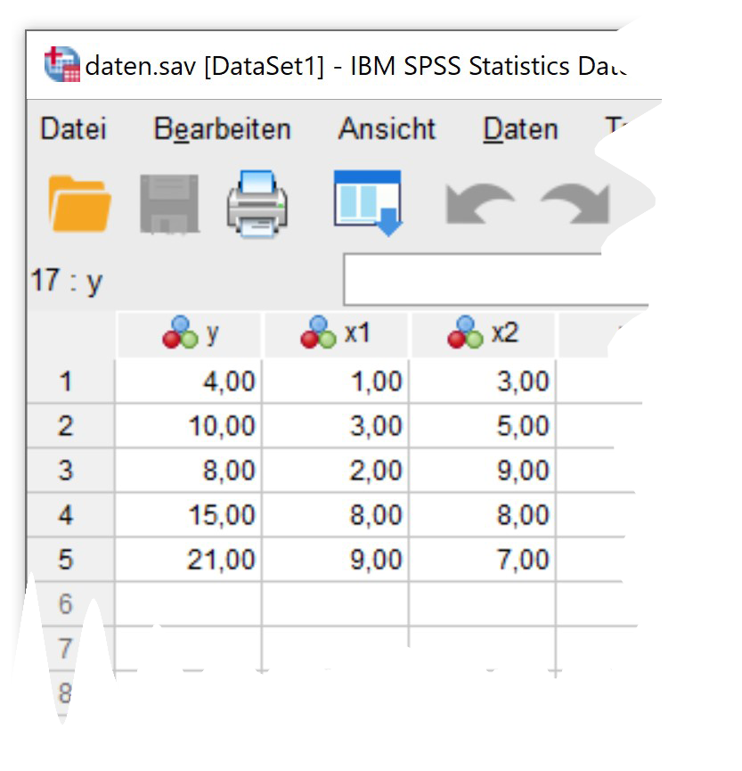

Teilaufgabe a

Berechnen Sie die Regressionskoeffizienten $\small b$ aufgrund des folgenden Ausdrucks: $\small b=\mathbf{(X'X)^{-1}X'y}$.

R
SPSS

b <- solve(t(X) %*% X) %*% t(X) %*% y
b

          [,1]
[1,] 2.9703433
[2,] 1.6942921
[3,] 0.1306114

MATRIX   
  
COMPUTE b= INV( T(x)*x )  * T(x)*y.
PRINT b.

END MATRIX.

Teilaufgabe b

Berechnen Sie die Residuen als $\small \mathbf{y-Xb}$ und den quadrierten Standardschätzfehler $\small s^2_e=\frac{1}{n-k-1}(y-\mathbf{X}b)'(y-\mathbf{X}b)$.

R
SPSS

res <- y-X %*% b
res

           [,1]
[1,] -1.0564696
[2,]  1.2937233
[3,]  0.4655698
[4,] -2.5695714
[5,]  1.8667479

Es ergeben sich $\small df=2$ Freiheitsgrade (durch $\small n-k$ aus $\small n=5$ Beobachtungen und $\small k=3$ Regressionskoeffizienten)

ve <- t(y-X %*% b) %*% (y-X %*% b) 
ve <- ve[1,1] / (5-3)
se <- sqrt(ve)
se

[1] 2.558715

MATRIX   
  
COMPUTE ve = T(y-x*b) * (y-x*b) / (5-3).
COMPUTE se=SQRT(ve).
PRINT se. 

END MATRIX.

Teilaufgabe c

Überprüfen Sie die Ergebnisse mit ~~SPSS~~ R~~EGRESSION~~.

R
SPSS

mdl_res <- summary(lm(y ~ x1 + x2, data = df)) 

mdl_res$coef

             Estimate Std. Error   t value   Pr(>|t|)
(Intercept) 2.9703433  3.5884923 0.8277413 0.49486217
x1          1.6942921  0.3927680 4.3137228 0.04976252
x2          0.1306114  0.5947684 0.2196005 0.84655791

mdl_res$residuals

         1          2          3          4          5 
-1.0564696  1.2937233  0.4655698 -2.5695714  1.8667479

mdl_res$sigma

[1] 2.558715

DATASET ACTIVATE DataSet1.
REGRESSION
  /MISSING LISTWISE
  /STATISTICS COEFF OUTS R ANOVA
  /CRITERIA=PIN(.05) POUT(.10)
  /NOORIGIN 
  /DEPENDENT y
  /METHOD=ENTER x1 x2.

Fußnoten

obgleich sie in R dennoch unter der Haube zum Einsatz kommen↩︎
die Notation von Matrizen wird durch Großbuchstaben in fetter Schreibweise realisiert↩︎
die Notation von Vektoren wird durch Kleinbuchstaben in fetter Schreibweise realisiert↩︎
es erfolgt keine gesonderte Notation, die Variablen für Skalare bzw. reelle Zahlen werden in Form lateinischer Kleinbuchstaben realisiert↩︎
engl. Identity-Matrix↩︎

Einführung

Terminologie

Spezielle Formen

Vektor (\(\small n\times 1\)- bzw. \(\small 1\times n\)-Matrix)

Skalar (\(\small 1\times 1\)-Matrix)

Quadratische Matrix

Symmetrische Matrix

Korrelationsmatrix

Diagonalmatrix

Einheitsmatrix

Nullmatrix

Umgeformte Matrizen

Transponierte Matrix

Transponierte Vektoren

Inverse Matrix

Rechnen mit Matrizen

Skalarmultiplikation

Matrixaddition

Matrixmultiplikation

Inneres und äußeres Produkt von Vektoren

Transponieren eines Produkts

Neutrales und inverses Element

Addition

Multiplikation

Determinante

Gesetzmäßigkeiten

Kommutativgesetz

Assoziativgesetz

Distributivgesetz

weitere Eigenschaften von Matrizen

Lineare Abhängigkeit

Determinanten und lineare Abhängigkeit

Rang einer Matrix

R/SPSS

R-Pakete

Base-R und SPSS Syntax

Übungsaufgaben

Aufgabe 1

Teilaufgabe a

Addition von Matrizen

Multiplikation mit einem Skalar

Subtraktion von Matrizen

Teilaufgabe b

Multiplikation von Matrizen

Teilaufgabe c

Aufgabe 2

Teilaufgabe a

Teilaufgabe b

Teilaufgabe c

Teilaufgabe d

Aufgabe 3

Teilaufgabe a

Teilaufgabe b

Aufgabe 4

Teilaufgabe a

Teilaufgabe b

Aufgabe 5

R

SPSS

Teilaufgabe a

Teilaufgabe b

Teilaufgabe c

Fußnoten