In this post I want to show how to create plots with R (2D and 3D) for different atlases, first. Second, I will demonstrate how plot personal data onto those plots. Therefore I use the data provided by Ganis et al. (2004). As this post serves also as a documentation for a short report¹, some details of the paper are mentioned here aswell.

Packages

library(here)
library(readr)

library(broom)
library(tibble)
library(dplyr)
library(tidyr)
library(magrittr)
library(ggplot2)

library(sp)
require(graphics)
require(grDevices)
library(colorRamps)
library(reshape2)

Atlas packages

Although there are other packages out there (e.g. the 📦 ggbrain-pacakge), we deal with the 📦 ggseg-package because

it builds on the known Grammar of Graphics, adapted in the 📦 ggplot2-package (Wickham, 2010)
provides everything we need to start (i.e. Desikan-Killany cortical atlas dk + Automatic subcortical segmentatio aseg)
with the 📦 ggsegExtra-package it provides a lot of addional atlases (see below)
custom atlases or coloring is possible and
everything can be ploted as well in 3D via the 📦 ggseg3d-package

# devtools::install_github("r-lib/vctrs")
# devtools::install_github("muschellij2/freesurfer")
# remotes::install_github("ggseg/ggsegExtra")

library(ggseg) 
library(ggseg3d)
library(ggsegExtra)

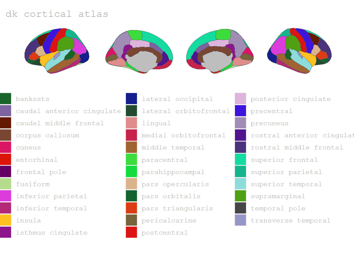
Desikan-Killany cortical atlas

The Desikan-Killany cortical atlas dk is provided as a basis by the 📦 ggseg-package. It contains 90 distinct brain regions (to access the regions and information see dk$data).

library(ggseg)

plot(dk)

As mentioned, the Desikan-Killany- and all the other cortical atlases can be viewed in 3D as well:

library(ggseg3d)

ggseg3d()

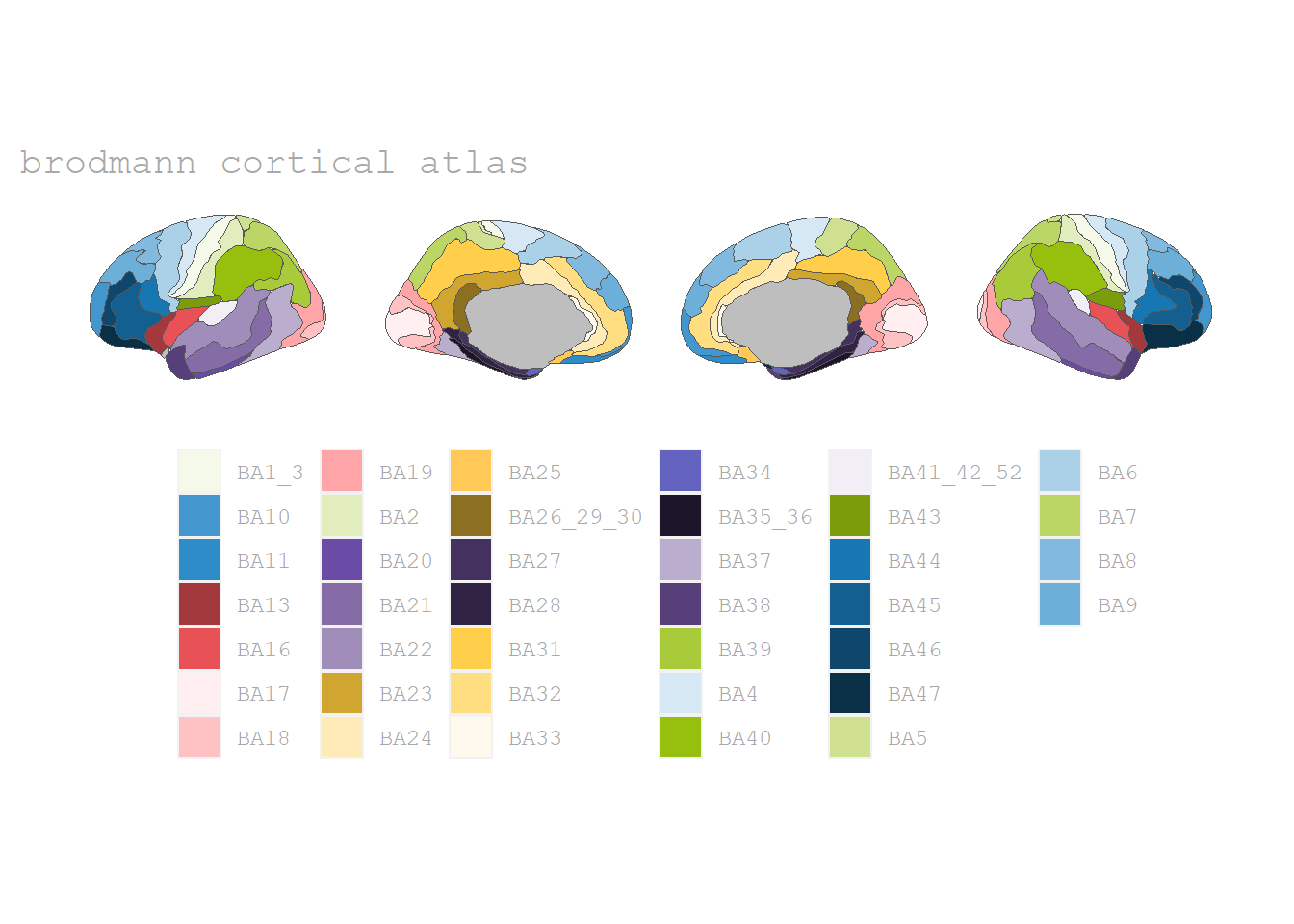
And as said, there are more atlases available, such as the Brodman areas:

Brodman ares

The Brodman ares (Brodman, 1909) are available in the 📦 ggsegBrodmann-package by Pijnenburg et al. (2021).

# remotes::install_github("ggseg/ggsegBrodmann")
library(ggsegBrodmann)

plot(brodmann)

Flechsig’ atlas of functional segregation

The atlas by Flechsig (1920) is a historical one that contains 46 regions, available via the 📦 ggsegFlechsig-package and also transfered to R by Pijnenburg et al. (2021).

# remotes::install_github("ggseg/ggsegFlechsig")

library(ggsegFlechsig)
library(ggsegExtra)

plot(flechsig)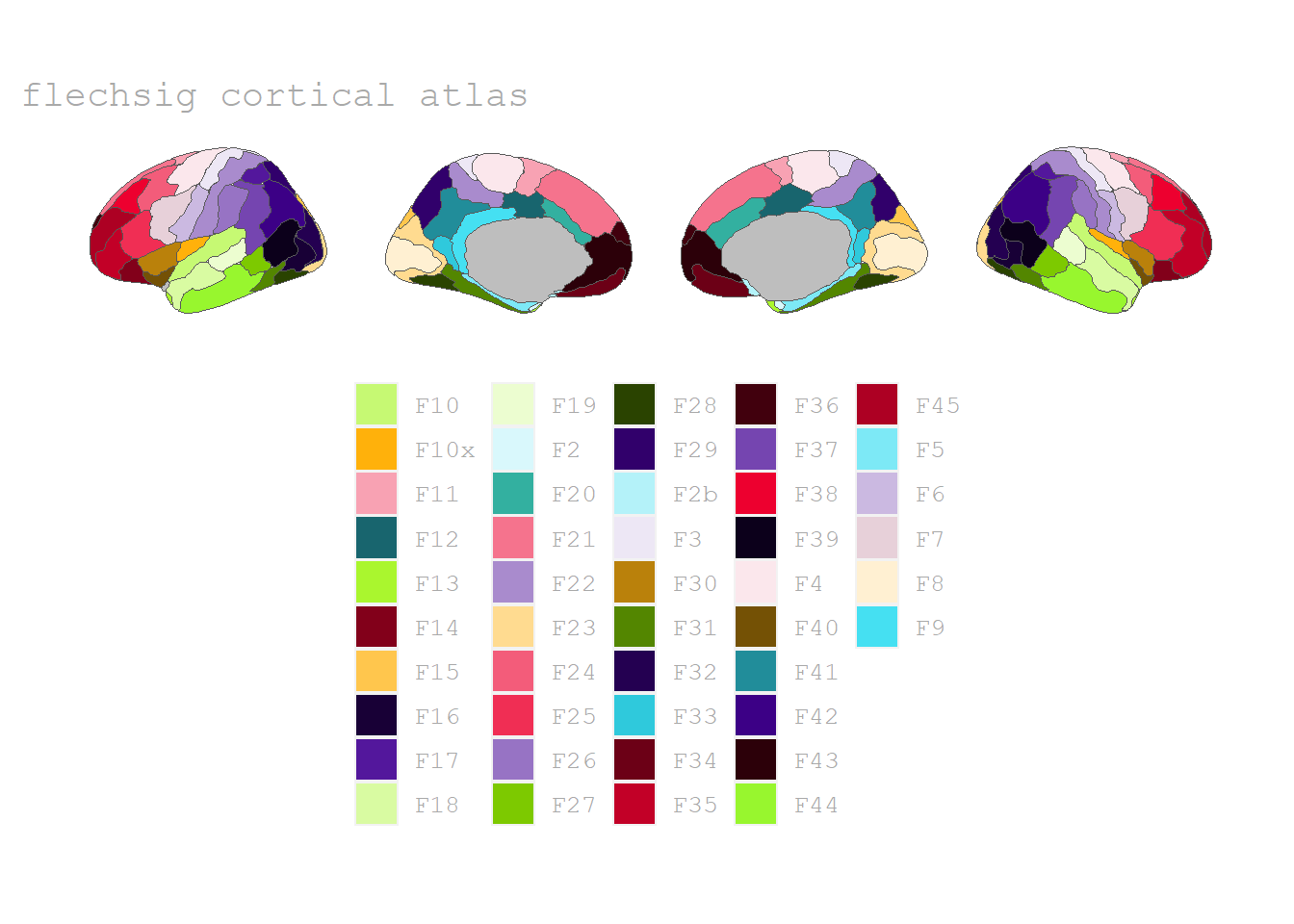

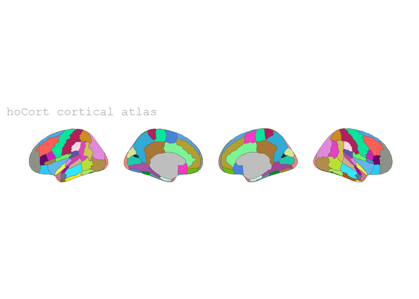
Harvard-Oxford cortical atlas

The Harvard-Oxford cortical atlas is the one we will use in the later example. For more see the paper of Makris et al. (2006).

# remotes::install_github("LCBC-UiO/ggsegHO")

library(ggsegHO)

plot(hoCort)

Example

Paper

To demonstrate how to color a given atlas with external data (e.g. information given by a research paper), I use the data provided by Ganis et al. (2004) in their article Brain areas underlying visual mental imagery and visual perception: an fMRI study.

The studies design can be sumed up as follows: participants had to learn a set of visual stimuli (white objects on black ground, e.g. a tree). Aferwards they underwent both conditions of the experiment: a) Perception (P) and b) Imagery (I) in seperate fMRI scans (counterbalanced).

During the P-condition they saw one of the known images per trail + heard a coresponding sound (e.g. the word tree). An accustic statement given 4.5 s later had to be confirmed (2AFC, e.g. wider than tall coded as W). I-condition was the same execpt subjects had to imagine the image (only sound, no image, eyes closed).

Reaction time data

(Non) responses and accuracy

On each trial, participants pressed one of two keys in response to the probe question. Participants were instructed not to press either key if they could not understand the name at the beginning of a trial because of scanner noise. Overall, the name was missed more often during the imagery than during the perception blocks (20.6% vs. 5.2%, respectively, F(1,14) = 22.32, p < 0.001).

Code

df_resp <- tribble(~"group",     ~"h_reaction_no",   
                    "imagery",    0.206,  
                    "perception", 0.052) %>% 
           mutate(h_reaction_yes = 1-h_reaction_no)

theme_set(theme_minimal())

df_resp %>% pivot_longer(cols = starts_with("h_reaction"),
                         names_to = "reaction",
                         names_prefix = "h_reaction_",
                         values_to = "h") %>% 
            mutate(label = paste0(round(h*100, 1), "%")) %>% 
            ggplot(aes(x = "", y = h, fill = reaction)) +
            geom_col(alpha = .8) +
            geom_label(aes(label = label),
                       position = position_stack(vjust = 0.5),
                       # size = 8,
                       show.legend = FALSE) +
            scale_fill_manual(values = c("lightcoral", "steelblue3")) +
            coord_polar(theta = "y") + 
            facet_wrap(~group) + 
            theme(# text = element_text(size = 30),
                  axis.title = element_blank(),
                  axis.text = element_blank())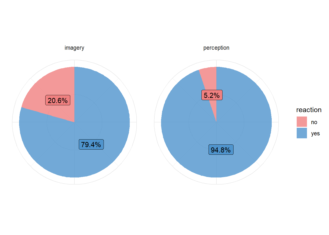

However, for the trials on which a response was made, accuracy was very high and did not differ between imagery and perception (96.2% vs. 97.3% correct, respectively, F(1,14) = 0.78, p>0.1)

Code

df_resp_acc <- tribble(~"condition", ~"h_reaction_correct",   
                       "imagery",    0.962,  
                       "perception", 0.973) %>% 
               mutate(h_reaction_incorrect = 1-h_reaction_correct) %>% 
               pivot_longer(cols = starts_with("h_reaction"),
                            names_to = "reaction",
                            names_prefix = "h_reaction_",
                            values_to = "h") %>% 
               mutate(label = paste0(round(h*100, 1), "%"))

df_resp_acc %>% ggplot(aes(x = reaction, y = h)) +
                geom_bar(aes(fill = reaction), 
                         show.legend = FALSE, alpha = .75,
                         stat = "identity", position = "dodge") + 
                scale_y_continuous("", labels = scales::label_percent()) +
                # scale_fill_viridis_d(option = "G", direction = -1) +
                scale_fill_manual(values = c("limegreen", "red")) +
                facet_wrap(~condition, scales = "free_x") + 
                # theme(text = element_text(size = 30)) +
                geom_label(aes(label = label), 
                               alpha = .85,
                               # size = 8,
                               position = position_stack(vjust = 0.5),
                               show.legend = FALSE)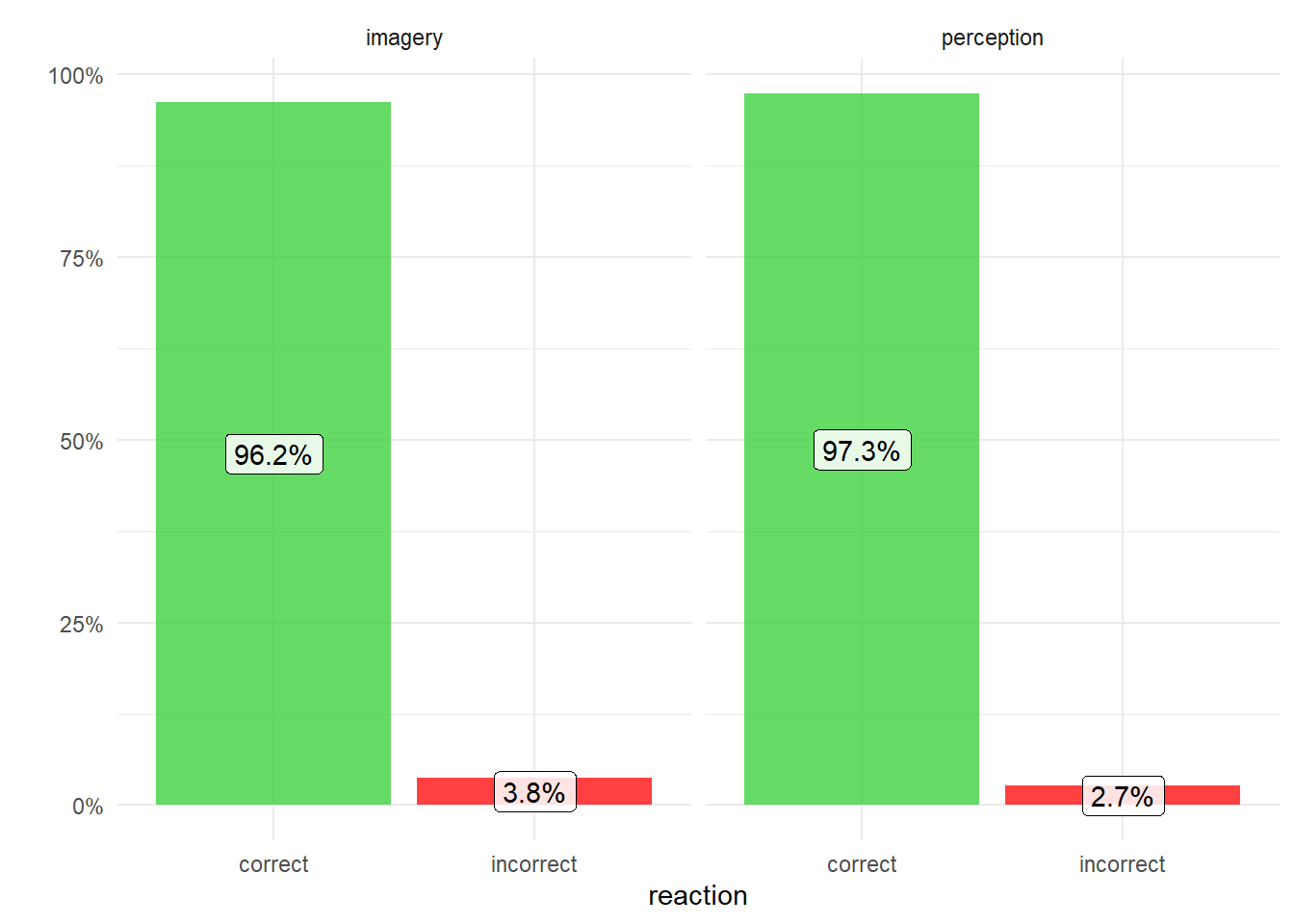

Reaction times

The response times (RTs) for correct trials were slower in the imagery condition than in the perception condition (medians: 1384 vs. 1232 ms, respectively, F(1,14) = 6.3, p = 0.025).

The same analysis was performed on a subgroup of 12 (out of 15) participants, excluding the 3 participants with the highest Imagery/Perception RT ratios. For this subgroup, there were no reliable differences between the median RTs in the two conditions (1299 vs. 1208 ms, respectively, F(1,14) = 2, p = 0.18)

Code

# tribble(~ "group", ~".y.", ~"group1", ~"group2",    ~"p", ~"p.adj.signif", ~"y.position",
#            1,       "RT",   "imagery", "perception", .025, "*",   1400,
#            2,       "RT",   "imagery", "perception", .18,  "ns.", 1320) -> stat.test

tribble(~"group", ~"condition", ~"RT", # Mdn
          1,       "imagery",    1384,
          1,       "perception", 1232,
          2,       "imagery",    1299,
          2,       "perception", 1208) -> df_mdn_rts

df_mdn_rts %>% mutate(group = factor(group, levels = c(1,2),
                                     labels = c("sample (n = 15)",
                                                "subsample (n = 12)"))) %>% 
               ggplot(aes(x = condition, y = RT)) + 
               geom_col(aes(fill = condition), show.legend = FALSE) +
               labs(y = "Mdn RT [ms]") +
               coord_cartesian(ylim = c(1100, 1500)) +
               facet_wrap(~ group) + 
             # ggpubr::stat_pvalue_manual(stat.test, label = "p", tip.length = 0.01)
             # theme(text = element_text(size = 30)) +
               scale_fill_viridis_d()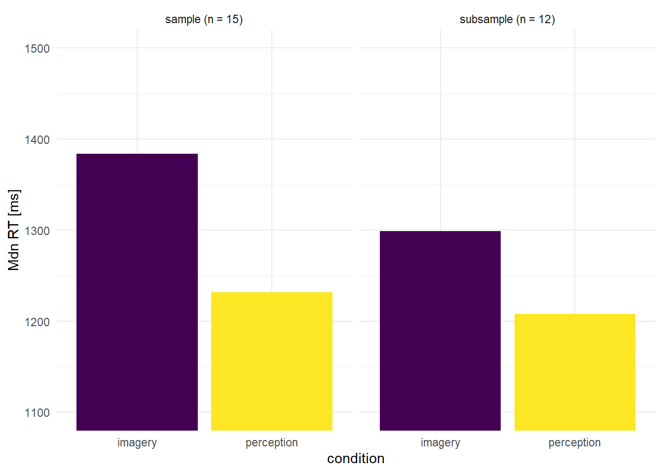

fMRI Data

Quantification of overlap

As the title already suggests, the brain regions that are activated during visual perception are compared to those activated during imagination. The authors quantify the amount of overlap (measured in voxels) as:

number of common voxels (C): voxels for which the contrast Perception vs. Imagery was n.s. and that exhibited a sig. activation change (rel. to baseline) during both imagery and perception

number of different voxels (D): voxels for which the contrast Perception vs. Imagery was significant and that exhibited a significant activation (rel. to baseline), in at least one condition

percentage of shared voxels (S): defined as:

\[S=100\times\frac{C}{C+D}\]

However, for all three quanfifications there are datasets (tables in the paper). I will deal with them in the following order²:

Common voxels (tab_3)
Different voxels (tab_4) and
Shared voxels (tab_2)

The tables in the paper are too long to be displayed on a PowerPoint slide in any meaningful way. I have therefore tried to transform the tables from long- to wide-shape. Nevertheless, you still can’t get any information from the tables. Therefore the tables are shown as bar-charts, where an activation in the corresponding areas is shown in color. The same colors are then used to color the corresponding brain areas. This should make it possible to see more quickly during the presentation which areas are relevant.

As said, all three of those datasets are included in this blog, however it is not neccessary to read the code for all three of them, so you may skip those parts and just look at the the results (i.e. shared voxels).

Possible contrasts

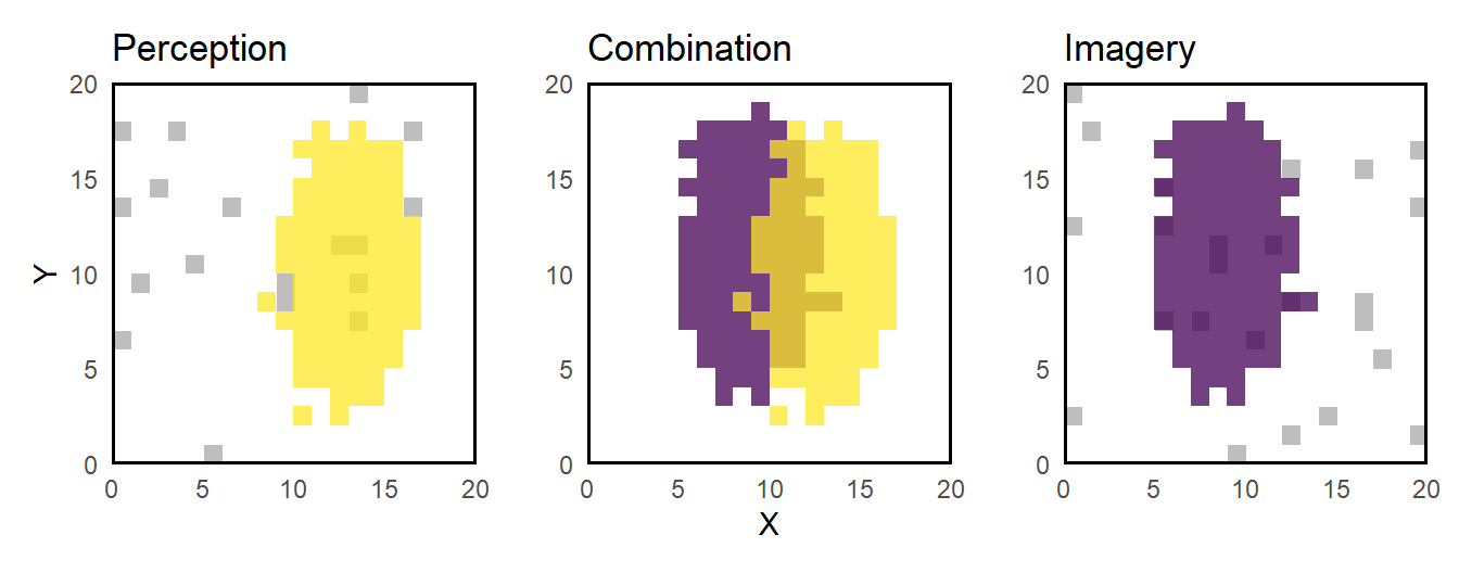
The authors only report significant contrasts (p = .0001). That’s why it’s important to understand which contrasts can exist in the first place. In visualization the gray patern symbolises the baseline activation, both activations (I and P) are sig. different from that, they are partly common and partly exclusive (what does not mean different).

S: Voxels are referred to as shared if they occur in any of the following conditions (C and D). They are computed according to the formula above, no differentiation is made with respect to any contrasts.
C: Voxels are referred to as common if a sig. activation change (rel. to baseline) is shown during both conditions, I and P, (i.e. [P>0, I>0] and [P<0, I<0]) and the same voxcels are activ in both conditions (i.e. [P-I=0]). Hence, there are only two possible contrasts: [P>0, I>0, P-I=0] and [P<0, I<0, P-I=0]
D: Voxels are referred to as different if a sig. activation change (rel. to baseline) is shown during at least one condition (i.e. [P>0, I=0], [P<0, I=0], [P=0, I>0], [P=0, I<0], [P>0, I>0], [P<0, I<0] but not [P<0, I>0] or [P>0, I<0]). Additionally, the contrast P vs I had to be significant (i.e. [P-I>0] or [P-I<0]). Hence, there are 12 possible contrasts:

\[ \small \begin{bmatrix} (P>0, I=0, P−I>0), & (P=0, I>0, P−I>0), & (P>0, I>0, P−I>0) \\ (P>0, I=0, P−I<0), & (P=0, I>0, P−I<0), & (P>0, I>0, P−I<0) \\ (P<0, I=0, P−I>0), & (P=0, I<0, P−I>0), & (P<0, I<0, P−I>0) \\ (P<0, I=0, P−I<0), & (P=0, I<0, P−I<0), & (P<0, I<0, P−I<0) \end{bmatrix} \]

Note. Significant differences are visible in only three of the shown 12 possible contrasts, i.e. (P>0, I=0, P−I>0), (P<0, I=0, P−I<0) and (P>0, I>0, P−I>0).

Reference dataframe

For beeing able to create a custom plot of the brain with the data provided above we have to make sure the names of the areas match with the names of the regions provided in the atlas (dk). Therefore we create a seperate dataframe. For the case when our data matched more then one reagion in the Desikan-Killiany Cortical Atlas we include two (or as many colums) as needed, e.g. we have data for the Middle frontal gyrus but since dk distinguished between rostral and middle frontal gyrus, we create two colums for that. For the other way arround (the atlas provides only one region for several colums of our data) we would choose a different atlas for the ones provided.

Harvard-Oxford cortical atlas Dict

Code

tribble(~"no", ~"region", ~"reg_abrv", 
1,                         "Angular Gyrus", "AG",
2,              "Central Opercular Cortex",  NA,
3,              "Frontal Operculum Cortex",  NA,
4,                "Frontal Orbital Cortex",  NA,
5,                          "Frontal Pole",  NA,
6,    "Heschl s Gyrus includes H1 and H2 ", "TransTG",
7,   "Inf. Frontal Gyrus pars opercularis", "IFG",
8,  "Inf. Frontal Gyrus pars triangularis", "IFG",
9,              "Inf. Temporal Gyrus ant.", "ITG",
10,            "Inf. Temporal Gyrus post.", "MOG",
11, "Inf. Temporal Gyrus temporooccipital", "MOG", # ~
12,                       "Insular Cortex", "Insula",
13,           "Lat. Occipital Cortex inf.", "IOG", 
14,       "Lat. Occipital Cortex superior", "SOG",
15,                   "Mid. Frontal Gyrus", "MFG",
16,             "Mid. Temporal Gyrus ant.", "MTG",
17,            "Mid. Temporal Gyrus post.", "MTG",
18, "Mid. Temporal Gyrus temporooccipital", "MTG",  #~
19,             "Occipital Fusiform Gyrus", "FG",
20,                       "Occipital Pole", "MOG", #~
21,            "Parietal Operculum Cortex", "IPL", # not good
22,                        "Planum Polare",  NA,
23,                     "Planum Temporale",  NA, 
24,                    "Postcentral Gyrus", "postCG",
25,                     "Precentral Gyrus", "PreCG",
26,                   "Sup. Frontal Gyrus", "SFG",
27,                 "Sup. Parietal Lobule", "SPL",
28,             "Sup. Temporal Gyrus ant.", "STG",
29,            "Sup. Temporal Gyrus post.", "STG",
30,             "Supramarginal Gyrus ant.", "SMG", 
31,            "Supramarginal Gyrus post.", "SMG",  
32,   "Temporal Occipital Fusiform Cortex", "FG",
33,                        "Temporal Pole",  NA,
34,                 "Cingulate Gyrus ant.", "AntCingG",
35,                "Cingulate Gyrus post.", "postCingG",
36,                        "Cuneal Cortex", "Cun",
37,                "Frontal Medial Cortex", "MeFG",
38,                "Intracalcarine Cortex",  NA,
39,        "Juxtapositional Lobule Cortex",  NA,
40,                        "Lingual Gyrus", "lingG",
41,                                   "NA",  NA,
42,                  "Paracingulate Gyrus", "CingG", # ? 
43,           "Parahippocampal Gyrus ant.", "paraHG",
44,          "Parahippocampal Gyrus post.", "paraHG",
45,                    "Precuneous Cortex", "preCuneus",
46,                   "Subcallosal Cortex",  NA,
47,                "Supracalcarine Cortex",  NA,
48,        "Temporal Fusiform Cortex ant.", "FG",
49,       "Temporal Fusiform Cortex post.", "FG"
) %>% select(-no) -> df_regio_abr2

#' nicht abgetragen:
#' Cerebellum - Cereb
#' LentNuc
#' Caudate
#' Claustrum
#' Thalamus
#' 
#' tab_3 %>% select(brain_region) %>% data.frame() %>% distinct() %>% filter(!brain_region %in% c("lingG", "Insula", "TransTG", "AG", "Cun", "postCingG", "AntCingG", "paraHG", "preCuneus", "postCG", "PreCG", "FG", "SFG", "IFG", "MFG", "MeFG", "SOG", "ITG", "MTG", "STG", "MOG", "SPL", "SMG", "CingG", "IPL", "IOG"))

Desikan-Killiany Cortical Atlas Dict (old)

Code

# old version
tribble(~"reg_abrv", ~"reg_name", ~"persp", ~"region", # region refers to dk region
        # FRONTAL
          "IFG",             "Inferior frontal gyrus",    "lateral", "pars orbitalis",  
          "IFG",             "Inferior frontal gyrus",    "lateral", "pars opercularis",
          "IFG",             "Inferior frontal gyrus",    "lateral", "pars triangularis",
          "MFG",             "Middle frontal gyrus",      "lateral", "caudal middle frontal",
          "MFG",             "Middle frontal gyrus",      "lateral", "rostral middle frontal",
          "SFG",           "Superior frontal gyrus",    "lateral", "superior frontal",
          "PreCG",     "Precentral gyrus",          "lateral", "precentral",
        # PARIETAL  
          "postCG",    "Postcentral gyrus",         "lateral", "postcentral",
          "IPL",       "Inferior parietal lobule",  "lateral", "inferior parietal",
          "SPL",       "Superior parietal lobule",  "lateral", "superior parietal",
          "AG",              "Angular gyrus",             "subcort", NA, # not good! lateral but not on map
          "SMG",         "Supramarginal gurus",       "lateral", "supramarginal",
        # TEMPORAL
          "ITG",             "Inferior temporal gyrus",   "lateral", "inferior temporal",
          "MTG",             "Middle temporal gyrus",     "lateral", "middle temporal", 
          "STG",             "Superior temporal gyrus",   "lateral", "superior temporal", 
          "STG",             "Superior temporal gyrus",   "lateral", "bankssts", # ~
          "TransTG",     "Transverse temporal gyrus", "lateral", "transverse temporal",
                        # = Heschl’sche Querwindungen
        # OCCIPITAL
          "SOG",             "Superior occipital gyrus",  "lateral", NA, #  
          "MOG",             "Middle occipital gyrus",    "lateral", "lateral occipital", 
          "MOG",             "Middle occipital gyrus",    "lateral", "pericalcarine",
          "IOG",             "Inferior occipital gyrus",  "lateral", NA, # ???
          
          "MeFG",            "Medial frontal gyrus",      "medial",  "paracentral", #??
                      # evtl. nur sup 
          "Insula",      "Insula",                    "lateral", "insula",  
            
          "AntCingG",    "Anterior cingulate gyrus",  "medial",  "caudal anterior cingulate", 
          "AntCingG",    "Anterior cingulate gyrus",  "medial",  "rostral anterior cingulate",
          "postCingG", "Posterior cingulate gyrus", "medial",    "isthmus cingulate",               
          
          "paraHG",      "Parahippocampal gyrus",     "medial",  "parahippocampal",
          "FG",        "Fusiform gyrus",            "medial",  "fusiform",
          "lingG",       "Lingual gyrus",             "medial",  "lingual",
          "preCuneus", "Precuneus",                 "medial",  "precuneus", 
          "Cun",           "Cuneus",                    "medial",    "cuneus",  
          "LentNuc",     "Lenticular nucleus",        "subcort", NA,
        # Ncl. lentiformis = Putamen + Globus pallidus
          "Claustrum", "Claustrum",                 "subcort", NA,
          "Thalamus",    "Thalamus",                  "subcort", NA,
          "Caudate",   "Caudate nucleus",           "subcort", NA,          
          "CingG",     "Cingulate gyrus",           "medial",    "posterior cingulate", # not sure what they mean since cing is present above   
          "Cereb",     "Cerebellum",                "subcort", NA) -> df_regio_abr
         # not sure if it's Cerebellum but can't be Cerebrum

# cf.:
# dk$data %>% data.frame() %>% select(region) %>% filter(!is.na(region)) %>% filter(grepl('dings', region))

Common voxels (C)

Altough the data is provided by a published article, there are some mistakes in the table for which we have to take account for, otherwise the plots won’t be correct. So after reading in the data we have to clean it (as shown below):

areas that have got different names in the other (upcoming) tables (e.g. ling vs. lingG should be the same)
areas that are named differently within the same datatable (e.g. Claustrum is once spelled Claustrun and since displayed as two differnt areas in the barcharts below)
additional problems, e.g. left and right postCG appears two times each in the table for shared voxels, what might be a) a mistake or b) because of missing talairach coordinates (x, y, z; cf. datatable 3 [below] and 4). We remove the doubled values since we do not know whether a or b is the case.
additional problem is caused not by the paper but its (Latex) format, i.e. the minus sign that is coded as a long minus (“—”) aka. “\002”.

Code

tab_3 <- read_table(here("data", "neuro", "tab_3.txt"),
                    col_types = list(side = col_character(),
                                     brain_region = col_character(),
                                     perc_overlap = col_double(),
                                     C_voxels = col_character(),
                                     x = col_character(),
                                     y = col_character(),
                                     z = col_character())) %>% 
         mutate(side = factor(side, levels = c("L", "R"), labels = c("left", "right")),
                brain_region = if_else(brain_region == "Claustrun", "Claustrum", 
                                       brain_region),
                C_voxels = stringr::str_replace_all(C_voxels, "\\*|\\(|\\)", "")) %>% 
         mutate_at(.vars = c("x", "y", "z"), 
                   ~stringr::str_replace_all(., "\\002", "-")) %>% 
         mutate_at(.vars = c("x", "y", "z"), 
                   ~stringr::str_replace_all(., ",", "")) %>% 
         mutate_at(.vars = c("C_voxels", "x", "y", "z"), as.numeric) # %>% 
         # distinct() # no! Values are distinct, cf. contrasts

tab_3 %<>% mutate(contrast = c(rep(1, 60), rep(2, 13))) %>%
           mutate(contrast = factor(contrast, levels = c(1, 2), 
                                    labels = c("P>0, I>0", "P<0, I<0"))) %>% 
           distinct()

Plots

(P>0, I>0) Activation stronger than baseline

Code

theme_set(theme_brain2())

tab_3 %>% filter(contrast == "P>0, I>0") %>% 
          # left_join(df_regio_abr, by = c("brain_region" = "reg_abrv")) %>% 
          left_join(df_regio_abr2, by = c("brain_region" = "reg_abrv")) %>% 
          rename(hemi = side) %>% 
          # mutate_at(scale, .vars = vars(C_voxels)) %>% 
          mutate(overlap = perc_overlap/100) %>% 
          select(-c(brain_region, # reg_name, 
                    perc_overlap)) %>% 
          filter(!is.na(region)) %>%
          ggplot() +
          scale_fill_viridis_c(option = "D", direction = 1)  +
          geom_brain(atlas = hoCort,
                     # atlas = dk, 
                     color = "white",
                     position = position_brain(side ~ hemi),
                     mapping = aes(fill = overlap)) +
          labs(fill = "overlap") + 
          theme(# legend.position = "none",
                plot.background = element_blank())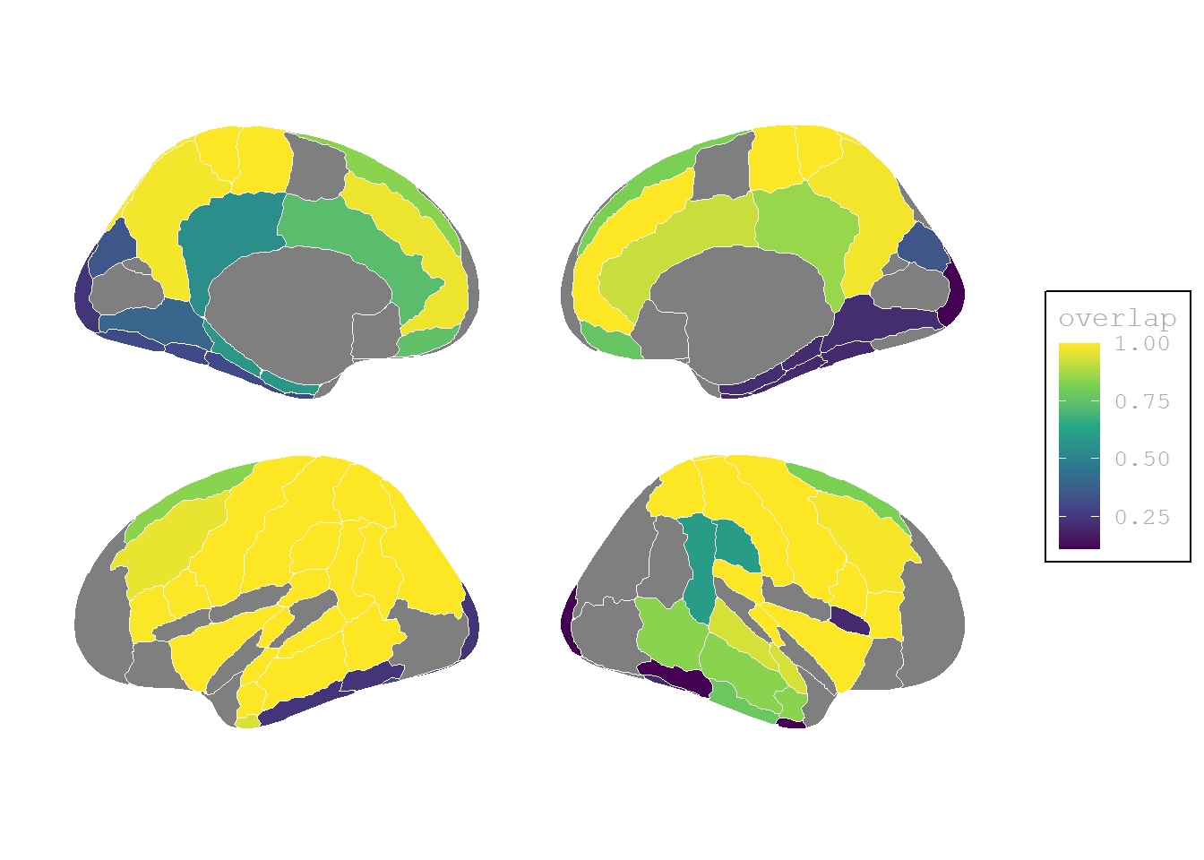

(P<0, I<0) Activation weaker than baseline

Code

theme_set(theme_brain2())

tab_3 %>% filter(contrast == "P<0, I<0") %>% 
        # left_join(df_regio_abr, by = c("brain_region" = "reg_abrv")) %>% 
          left_join(df_regio_abr2, by = c("brain_region" = "reg_abrv")) %>%
          rename(hemi = side) %>% 
        # mutate_at(scale, .vars = vars(C_voxels)) %>% 
          mutate(overlap = perc_overlap/100) %>% 
          select(-c(brain_region, # reg_name, 
                    perc_overlap)) %>% 
          filter(!is.na(region)) %>%
          ggplot() +
          scale_fill_viridis_c(option = "D", direction = 1)  +
          geom_brain(atlas = hoCort, # atlas = dk, 
                     color = "white",
                     position = position_brain(side ~ hemi),
                     mapping = aes(fill = overlap)) +
          labs(fill = "overlap") + 
          theme(# legend.position = "none",
                plot.background = element_blank())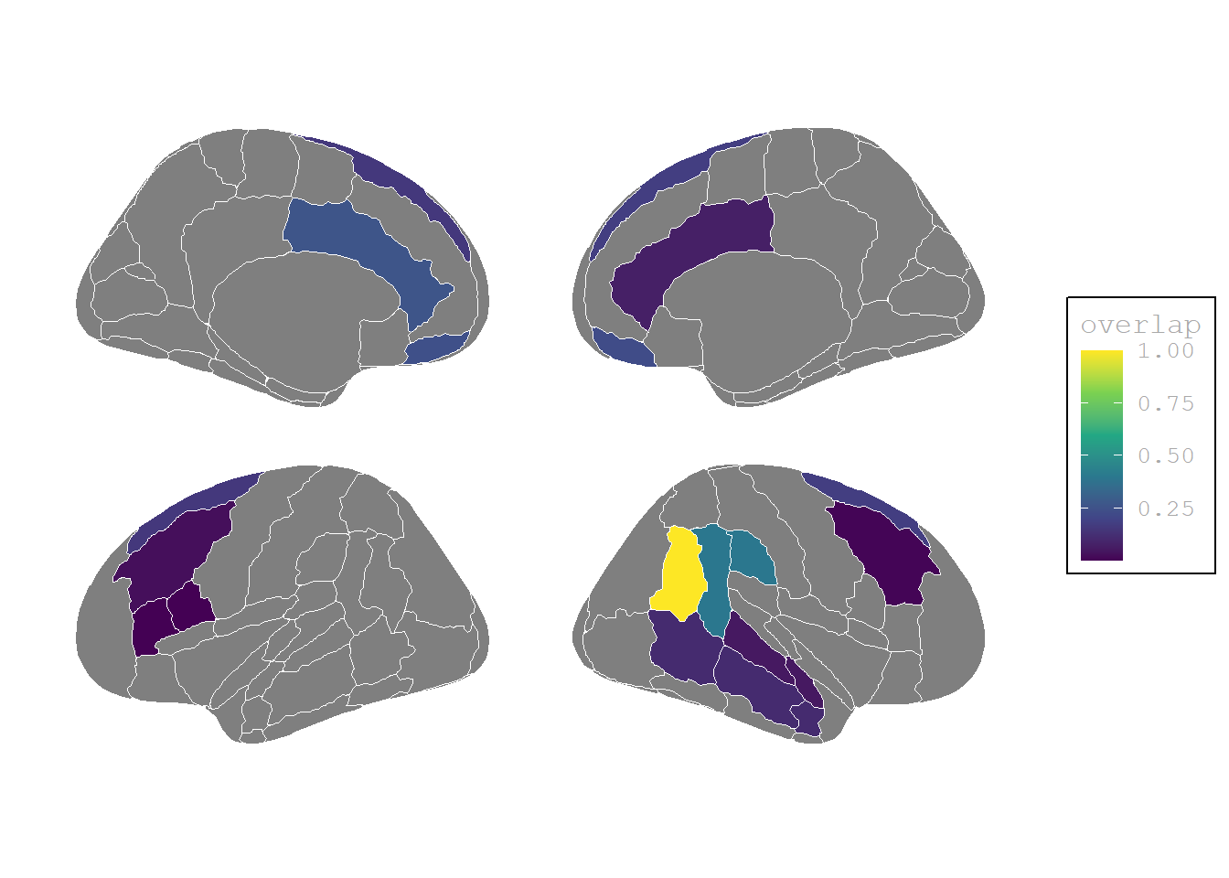

Activation barchart

Only significant contrasts are shown (p = 0.0001), i.e. activation was a) significant higher than at the baseline (P>0, I>0) or significant lower (P<0, I<0) than the baseline for both conditions, but the activation patters were not significant different than zero, i.e. they were similar (P-I=0)

Code

theme_set(theme_minimal())

# df_regio_abr %>% select(reg_abrv, persp) %>% 
#                  distinct() %>% 
#                  right_join(tab_3, by = c("reg_abrv" = "brain_region")) %>% 
#           # filter(persp != "subcort") %>% 
#           mutate(rel_overlap = perc_overlap/100) %>% 
# # tab_3 %>% mutate(rel_overlap = perc_overlap/100) %>% 
#           ggplot(aes(x = reorder(reg_abrv, rel_overlap), 
#                      y = rel_overlap, fill = rel_overlap)) + 
#           geom_bar(stat = "identity") + 
#           scale_fill_viridis_c(option = "viridis", guide = "none", direction = 1) +
#           scale_y_continuous("common voxels", labels = scales::label_percent()) +
#           facet_grid(contrast~side, scales = "free", space = "free", drop = TRUE) +
#         # theme(axis.ticks.y = element_blank()) +
#           labs(x = "brain region") + 
#           theme(text = element_text(size = 20),
#                 panel.spacing = unit(0.5, "cm")) +
#           coord_flip() 
#         #  theme_minimal()

tab_3 %>% mutate(rel_overlap = perc_overlap/100) %>% 
          ggplot(aes(x = reorder(brain_region, rel_overlap), 
                     y = rel_overlap, fill = rel_overlap)) + 
          geom_bar(stat = "identity") + 
          scale_fill_viridis_c(option = "viridis", guide = "none", direction = 1) +
          scale_y_continuous("common voxels", labels = scales::label_percent()) +
          facet_grid(contrast~side, scales = "free", space = "free", drop = TRUE) +
        # theme(axis.ticks.y = element_blank()) +
          labs(x = "brain region") + 
          theme(# text = element_text(size = 20),
                panel.spacing = unit(0.5, "cm")) +
          coord_flip() -> vxl_chrt_c
vxl_chrt_c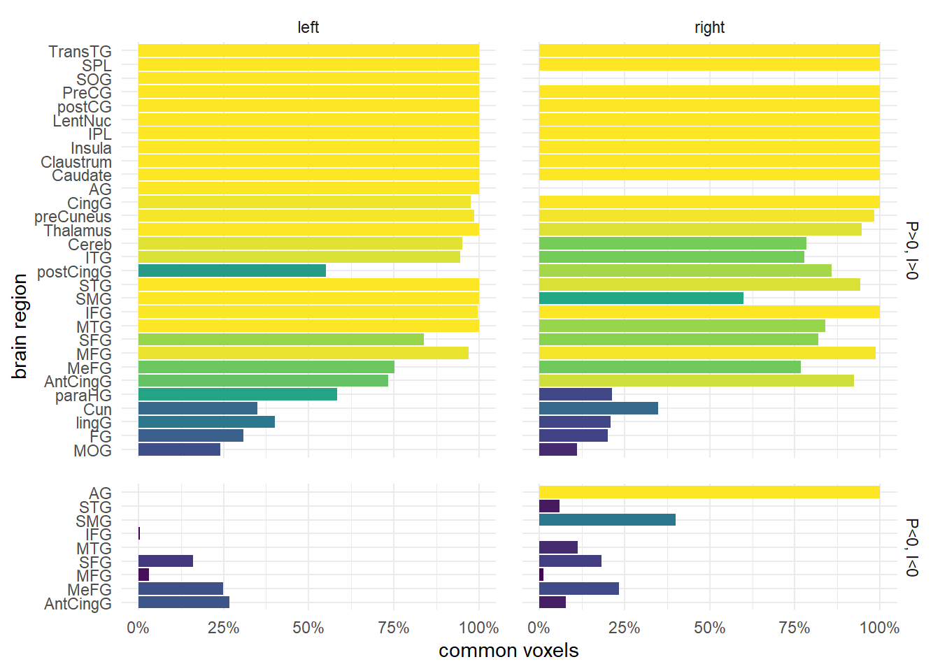

Table C voxels

long to wide tab

Code

tab_3 %>% pivot_wider(names_from = "side", 
                      values_from = c("perc_overlap", "C_voxels", "x", "y", "z")) %>% 
          relocate("C_voxels_left", .before = "perc_overlap_left") %>% 
          relocate("C_voxels_right", .before = "perc_overlap_right") %>% 
          relocate("y_left", .after = "x_left") %>%  
          relocate("z_left", .after = "y_left") -> tab_3_wide

df_regio_abr %>% select(c(reg_abrv, reg_name, persp)) %>% 
                 distinct() %>% 
                 right_join(tab_3_wide, by = c("reg_abrv" = "brain_region")) %>% 
                 mutate(brain_region = paste0(reg_name, " (", reg_abrv, ")")) %>%
               # filter(persp != "lateral") %>% 
                 select(-c(reg_name, persp, reg_abrv)) %>% 
# tab_3_wide %>% left_join(df_regio_abr, by = c("brain_region" = "reg_abrv")) %>% 
#                mutate(brain_region = paste0(reg_name, " (", brain_region, ")")) %>%
#                select(-c(reg_name, persp)) %>% 
               gt(rowname_col = "brain_region",
                  groupname_col = "contrast") %>% 
               tab_stubhead(label = "Contrast") %>% 
               tab_spanner(label = "left", 
                           columns = c(C_voxels_left, perc_overlap_left, x_left,    y_left, z_left)) %>% 
               tab_spanner(label = "right", 
                           columns = c(C_voxels_right, perc_overlap_right, x_right, y_right, z_right)) %>% 
               # tab_spanner(label = "left", 
               #             columns = c(x_left,    y_left, z_left)) %>% 
               # tab_spanner(label = "right", 
               #             columns = c(x_right,   y_right, z_right)) %>% 
             # cols_merge(columns = c(S_voxels_left, perc_overlap_left),
             #            pattern = "{1} ({2})") %>%
             # cols_merge(columns = c(S_voxels_right,   perc_overlap_right),
             #            pattern = "{1} ({2})") %>%
             # cols_label(S_voxels_left = "S voxels (%)",
             #            S_voxels_right = "S voxels (%)")
               cols_label(C_voxels_left = "C voxels",
                          perc_overlap_left = "%",
                          C_voxels_right = "C voxels",
                          perc_overlap_right = "%",
                          x_left = "x", y_left = "y", z_left = "z",
                          x_right = "x", y_right = "y", z_right = "z") %>% 
               sub_missing() %>% 
               cols_align(align = "center", columns = everything()) %>% 
               as_raw_html()

Contrast	left					right
Contrast	C voxels	%	x	y	z	C voxels	%	x	y	z
P>0, I>0
Inferior frontal gyrus (IFG)	241	99.6	-45	20	13	146	100.0	45	16	14
Middle frontal gyrus (MFG)	325	96.9	-37	22	30	250	98.8	37	21	31
Superior frontal gyrus (SFG)	93	83.9	-20	34	33	88	81.8	20	38	30
Precentral gyrus (PreCG)	231	100.0	-43	-5	36	80	100.0	42	0	33
Postcentral gyrus (postCG)	157	100.0	-49	-23	39	31	100.0	47	-24	35
Inferior parietal lobule (IPL)	206	100.0	-44	-40	40	91	100.0	40	-43	43
Superior parietal lobule (SPL)	80	100.0	-28	-61	51	53	100.0	28	-61	50
Angular gyrus (AG)	11	100.0	-33	-60	34	—	—	—	—	—
Supramarginal gurus (SMG)	47	100.0	-47	-44	33	15	60.0	40	-43	35
Inferior temporal gyrus (ITG)	18	94.4	-55	-57	-6	9	77.8	52	-49	-13
Middle temporal gyrus (MTG)	94	100.0	-51	-52	3	62	83.9	51	-41	0
Superior temporal gyrus (STG)	226	100.0	-54	-25	9	173	94.2	52	-24	7
Transverse temporal gyrus (TransTG)	18	100.0	-49	-22	12	20	100.0	47	-24	12
Superior occipital gyrus (SOG)	2	100.0	-32	-75	30	—	—	—	—	—
Middle occipital gyrus (MOG)	58	24.1	-51	-63	5	90	11.1	49	-62	6
Medial frontal gyrus (MeFG)	113	75.2	-8	10	45	90	76.7	8	12	45
Insula (Insula)	99	100.0	-38	-1	11	87	100.0	39	4	7
Anterior cingulate gyrus (AntCingG)	30	73.3	-9	28	20	13	92.3	8	25	23
Posterior cingulate gyrus (postCingG)	20	55.0	-4	-36	20	14	85.7	3	-37	20
Parahippocampal gyrus (paraHG)	12	58.3	-17	-34	1	14	21.4	18	-28	-4
Fusiform gyrus (FG)	13	30.8	-51	-54	-14	15	20.0	46	-53	-12
Lingual gyrus (lingG)	45	40.0	-4	-86	-5	86	20.9	6	-91	-7
Precuneus (preCuneus)	159	98.7	-18	-66	43	121	98.3	16	-65	44
Cuneus (Cun)	43	34.9	-12	-81	14	86	34.9	5	-86	9
Lenticular nucleus (LentNuc)	102	100.0	-23	-2	3	55	100.0	22	1	3
Claustrum (Claustrum)	29	100.0	-30	5	3	20	100.0	28	16	4
Thalamus (Thalamus)	114	100.0	-10	-18	8	95	94.7	8	-17	8
Caudate nucleus (Caudate)	50	100.0	-14	0	14	46	100.0	12	3	12
Cingulate gyrus (CingG)	127	97.6	-7	5	35	108	100.0	7	6	35
Cerebellum (Cereb)	41	95.1	-10	-49	-9	46	78.3	11	-53	-12
P<0, I<0
Inferior frontal gyrus (IFG)	241	0.4	-54	23	-12	—	—	—	—	—
Middle frontal gyrus (MFG)	325	3.1	-26	28	38	250	1.2	49	20	40
Superior frontal gyrus (SFG)	93	16.1	-17	44	37	88	18.2	15	44	38
Angular gyrus (AG)	—	—	—	—	—	3	100.0	50	-58	33
Supramarginal gurus (SMG)	—	—	—	—	—	15	40.0	45	-54	31
Middle temporal gyrus (MTG)	—	—	—	—	—	62	11.3	48	-51	16
Superior temporal gyrus (STG)	—	—	—	—	—	173	5.8	45	-56	26
Medial frontal gyrus (MeFG)	113	24.8	-4	52	7	90	23.3	4	53	16
Anterior cingulate gyrus (AntCingG)	30	26.7	-6	33	9	13	7.7	18	35	20

contrasts side by side

Code

df_regio_abr %>% select(c(reg_abrv, reg_name, persp)) %>% 
                 distinct() %>% 
                 right_join(tab_3, by = c("reg_abrv" = "brain_region")) %>% 
                 mutate(brain_region = paste0(reg_name, " (", reg_abrv, ")"),
                        contrast = recode_factor(contrast, "P>0, I>0" = "A", 
                                                           "P<0, I<0" = "B")) %>%
                                                  # labels = c("P>0, I>0", "P<0, I<0"))) 
               # filter(persp != "lateral") %>% 
                 select(-c(reg_name, persp, reg_abrv)) %>% 
                 pivot_wider(values_from = c(perc_overlap, C_voxels, x, y, z), 
                             names_from = "contrast", values_fill = NA) %>% 
                 gt(rowname_col = "brain_region",
                    groupname_col = "side") %>% 
                 tab_stubhead(label = "Brain region") %>% 
                 tab_spanner(label = "P>0, I>0", 
                             columns = ends_with("_A")) %>% 
                 tab_spanner(label = "P<0, I<0", 
                             columns = ends_with("_B")) %>% 
                 cols_label(C_voxels_A = "C voxels",
                            perc_overlap_A = "%",
                            C_voxels_B = "C voxels",
                            perc_overlap_B = "%",
                            x_A = "x", y_A = "y", z_A = "z",
                            x_B = "x", y_B = "y", z_B = "z") %>% 
                 sub_missing() %>% 
                 cols_align(align = "center", columns = everything()) %>% 
                 as_raw_html()

Brain region	P>0, I>0					P<0, I<0
Brain region	%	C voxels	x	y	z	%	C voxels	x	y	z
left
Inferior frontal gyrus (IFG)	99.6	241	-45	20	13	0.4	241	-54	23	-12
Middle frontal gyrus (MFG)	96.9	325	-37	22	30	3.1	325	-26	28	38
Superior frontal gyrus (SFG)	83.9	93	-20	34	33	16.1	93	-17	44	37
Precentral gyrus (PreCG)	100.0	231	-43	-5	36	—	—	—	—	—
Postcentral gyrus (postCG)	100.0	157	-49	-23	39	—	—	—	—	—
Inferior parietal lobule (IPL)	100.0	206	-44	-40	40	—	—	—	—	—
Superior parietal lobule (SPL)	100.0	80	-28	-61	51	—	—	—	—	—
Angular gyrus (AG)	100.0	11	-33	-60	34	—	—	—	—	—
Supramarginal gurus (SMG)	100.0	47	-47	-44	33	—	—	—	—	—
Inferior temporal gyrus (ITG)	94.4	18	-55	-57	-6	—	—	—	—	—
Middle temporal gyrus (MTG)	100.0	94	-51	-52	3	—	—	—	—	—
Superior temporal gyrus (STG)	100.0	226	-54	-25	9	—	—	—	—	—
Transverse temporal gyrus (TransTG)	100.0	18	-49	-22	12	—	—	—	—	—
Superior occipital gyrus (SOG)	100.0	2	-32	-75	30	—	—	—	—	—
Middle occipital gyrus (MOG)	24.1	58	-51	-63	5	—	—	—	—	—
Medial frontal gyrus (MeFG)	75.2	113	-8	10	45	24.8	113	-4	52	7
Insula (Insula)	100.0	99	-38	-1	11	—	—	—	—	—
Anterior cingulate gyrus (AntCingG)	73.3	30	-9	28	20	26.7	30	-6	33	9
Posterior cingulate gyrus (postCingG)	55.0	20	-4	-36	20	—	—	—	—	—
Parahippocampal gyrus (paraHG)	58.3	12	-17	-34	1	—	—	—	—	—
Fusiform gyrus (FG)	30.8	13	-51	-54	-14	—	—	—	—	—
Lingual gyrus (lingG)	40.0	45	-4	-86	-5	—	—	—	—	—
Precuneus (preCuneus)	98.7	159	-18	-66	43	—	—	—	—	—
Cuneus (Cun)	34.9	43	-12	-81	14	—	—	—	—	—
Lenticular nucleus (LentNuc)	100.0	102	-23	-2	3	—	—	—	—	—
Claustrum (Claustrum)	100.0	29	-30	5	3	—	—	—	—	—
Thalamus (Thalamus)	100.0	114	-10	-18	8	—	—	—	—	—
Caudate nucleus (Caudate)	100.0	50	-14	0	14	—	—	—	—	—
Cingulate gyrus (CingG)	97.6	127	-7	5	35	—	—	—	—	—
Cerebellum (Cereb)	95.1	41	-10	-49	-9	—	—	—	—	—
right
Inferior frontal gyrus (IFG)	100.0	146	45	16	14	—	—	—	—	—
Middle frontal gyrus (MFG)	98.8	250	37	21	31	1.2	250	49	20	40
Superior frontal gyrus (SFG)	81.8	88	20	38	30	18.2	88	15	44	38
Precentral gyrus (PreCG)	100.0	80	42	0	33	—	—	—	—	—
Postcentral gyrus (postCG)	100.0	31	47	-24	35	—	—	—	—	—
Inferior parietal lobule (IPL)	100.0	91	40	-43	43	—	—	—	—	—
Superior parietal lobule (SPL)	100.0	53	28	-61	50	—	—	—	—	—
Angular gyrus (AG)	—	—	—	—	—	100.0	3	50	-58	33
Supramarginal gurus (SMG)	60.0	15	40	-43	35	40.0	15	45	-54	31
Inferior temporal gyrus (ITG)	77.8	9	52	-49	-13	—	—	—	—	—
Middle temporal gyrus (MTG)	83.9	62	51	-41	0	11.3	62	48	-51	16
Superior temporal gyrus (STG)	94.2	173	52	-24	7	5.8	173	45	-56	26
Transverse temporal gyrus (TransTG)	100.0	20	47	-24	12	—	—	—	—	—
Middle occipital gyrus (MOG)	11.1	90	49	-62	6	—	—	—	—	—
Medial frontal gyrus (MeFG)	76.7	90	8	12	45	23.3	90	4	53	16
Insula (Insula)	100.0	87	39	4	7	—	—	—	—	—
Anterior cingulate gyrus (AntCingG)	92.3	13	8	25	23	7.7	13	18	35	20
Posterior cingulate gyrus (postCingG)	85.7	14	3	-37	20	—	—	—	—	—
Parahippocampal gyrus (paraHG)	21.4	14	18	-28	-4	—	—	—	—	—
Fusiform gyrus (FG)	20.0	15	46	-53	-12	—	—	—	—	—
Lingual gyrus (lingG)	20.9	86	6	-91	-7	—	—	—	—	—
Precuneus (preCuneus)	98.3	121	16	-65	44	—	—	—	—	—
Cuneus (Cun)	34.9	86	5	-86	9	—	—	—	—	—
Lenticular nucleus (LentNuc)	100.0	55	22	1	3	—	—	—	—	—
Claustrum (Claustrum)	100.0	20	28	16	4	—	—	—	—	—
Thalamus (Thalamus)	94.7	95	8	-17	8	—	—	—	—	—
Caudate nucleus (Caudate)	100.0	46	12	3	12	—	—	—	—	—
Cingulate gyrus (CingG)	100.0	108	7	6	35	—	—	—	—	—
Cerebellum (Cereb)	78.3	46	11	-53	-12	—	—	—	—	—

Different voxels (D)

Code

tab_4 <- read_table(here("data", "neuro", "tab_4.txt"),
                    col_types = list(side = col_character(),
                                     brain_region = col_character(),
                                     perc_overlap = col_double(),
                                     D_voxels = col_character(),
                                     x = col_character(),
                                     y = col_character(),
                                     z = col_character())) %>% 
         mutate(side = factor(side, levels = c("L", "R"), 
                              labels = c("left", "right")),
                brain_region = if_else(brain_region == "Claustrun", 
                                       "Claustrum", brain_region),
                D_voxels = stringr::str_replace_all(D_voxels, "\\*|\\(|\\)", "")) %>% 
         mutate_at(.vars = c("x", "y", "z"), 
                   ~stringr::str_replace_all(., "\\002", "-")) %>% 
         mutate_at(.vars = c("x", "y", "z"), 
                   ~stringr::str_replace_all(., ",", "")) %>% 
         mutate_at(.vars = c("D_voxels", "x", "y", "z"), as.numeric) # %>% 
         # distinct() # no! Values are distinct, cf. contrasts

tab_4 %<>% mutate(contrast = c(rep(1, 3), rep(2, 19), rep(3, 4))) %>% 
           mutate(contrast = factor(contrast, levels = c(1:3), 
                  labels = c("...,I>0,...", "P>0, I=0, P-I>0", "P<0,...,P-I<0")))

Plots

Activation maps

The authors report only three contrasts with significantly different activation, i.e. (P>0, I=0, P−I>0), (P<0, I=0, P−I<0) and (P>0, I>0, P−I>0). For the last two of them this is only true for few areas:

(P>0, I=0, P−I>0)

Code

theme_set(theme_brain2())

tab_4 %>% filter(contrast == "P>0, I=0, P-I>0") %>% 
        # left_join(df_regio_abr, by = c("brain_region" = "reg_abrv")) %>% 
          left_join(df_regio_abr2, by = c("brain_region" = "reg_abrv")) %>%
          rename(hemi = side) %>% 
        # mutate_at(scale, .vars = vars(C_voxels)) %>% 
          mutate(overlap = perc_overlap/100) %>% 
          select(-c(brain_region, # reg_name, 
                    perc_overlap)) %>% 
          filter(!is.na(region)) %>% 
          ggplot() +
          scale_fill_viridis_c(option = "D", direction = 1)  +
          geom_brain(atlas = hoCort, # atlas = dk, 
                     color = "white",
                     position = position_brain(side ~ hemi),
                     mapping = aes(fill = overlap)) +
          labs(fill = "overlap") + 
          theme(# legend.position = "none",
                plot.background = element_blank())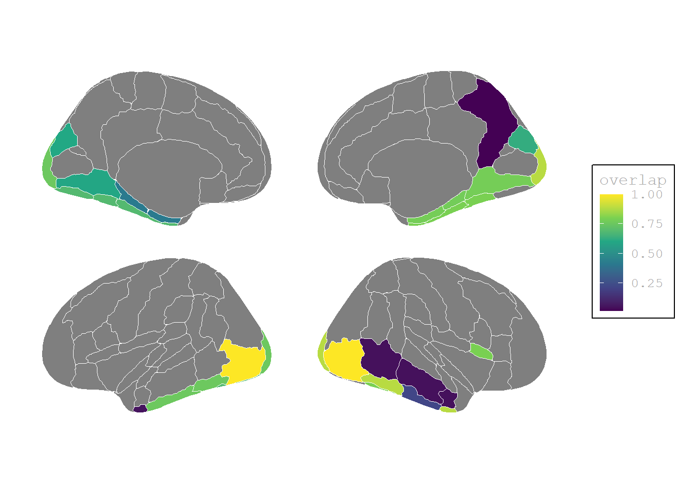

(P<0, I=0, P−I<0)

Code

theme_set(theme_brain2())

tab_4 %>% filter(contrast == "P<0,...,P-I<0") %>% 
        # left_join(df_regio_abr, by = c("brain_region" = "reg_abrv")) %>% 
          left_join(df_regio_abr2, by = c("brain_region" = "reg_abrv")) %>%
          rename(hemi = side) %>% 
        # mutate_at(scale, .vars = vars(C_voxels)) %>% 
          mutate(overlap = perc_overlap/100) %>% 
          select(-c(brain_region, # reg_name, 
                    perc_overlap)) %>% 
# bind_rows(data.frame(hemi = "right", region = "Temporal Fusiform Cortex ant.", overlap = 1)) %>% 
          filter(!is.na(region)) %>%
          ggplot() +
          scale_fill_viridis_c(option = "D", direction = 1)  +
          geom_brain(atlas = hoCort, # atlas = dk, 
                     color = "white",
                     position = position_brain(side ~ hemi),
                     mapping = aes(fill = overlap)) +
          labs(fill = "overlap") + 
          theme(# legend.position = "none",
                plot.background = element_blank())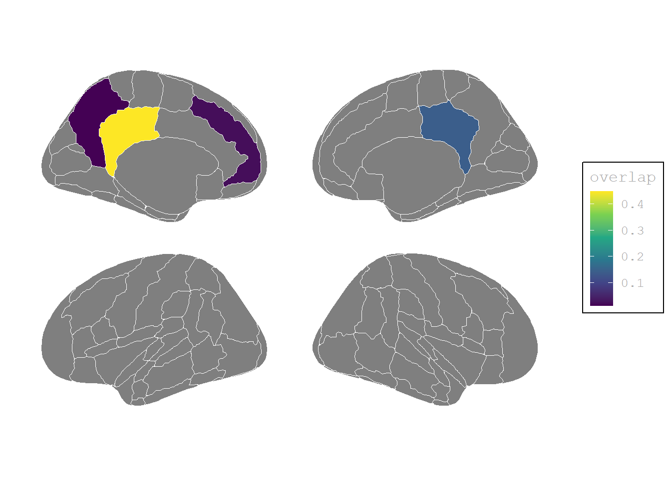

(P>0, I>0, P−I>0)

Code

theme_set(theme_brain2())

tab_4 %>% filter(contrast == "...,I>0,...") %>% 
        # left_join(df_regio_abr, by = c("brain_region" = "reg_abrv")) %>% 
          left_join(df_regio_abr2, by = c("brain_region" = "reg_abrv")) %>%
          rename(hemi = side) %>% 
        # mutate_at(scale, .vars = vars(C_voxels)) %>% 
          mutate(overlap = perc_overlap/100) %>% 
          select(-c(brain_region, # reg_name, 
                    perc_overlap)) %>% 
# bind_rows(data.frame(hemi = "right", region = "Temporal Fusiform Cortex ant.", overlap = 1)) %>% 
          filter(!is.na(region)) %>%
          ggplot() +
          scale_fill_viridis_c(option = "D", direction = 1, begin = 0, end = 1)  +
          geom_brain(atlas = hoCort, # atlas = dk, 
                     color = "white",
                     position = position_brain(side ~ hemi),
                     mapping = aes(fill = overlap)) +
          labs(fill = "overlap") + 
          theme(# legend.position = "none",
                plot.background = element_blank())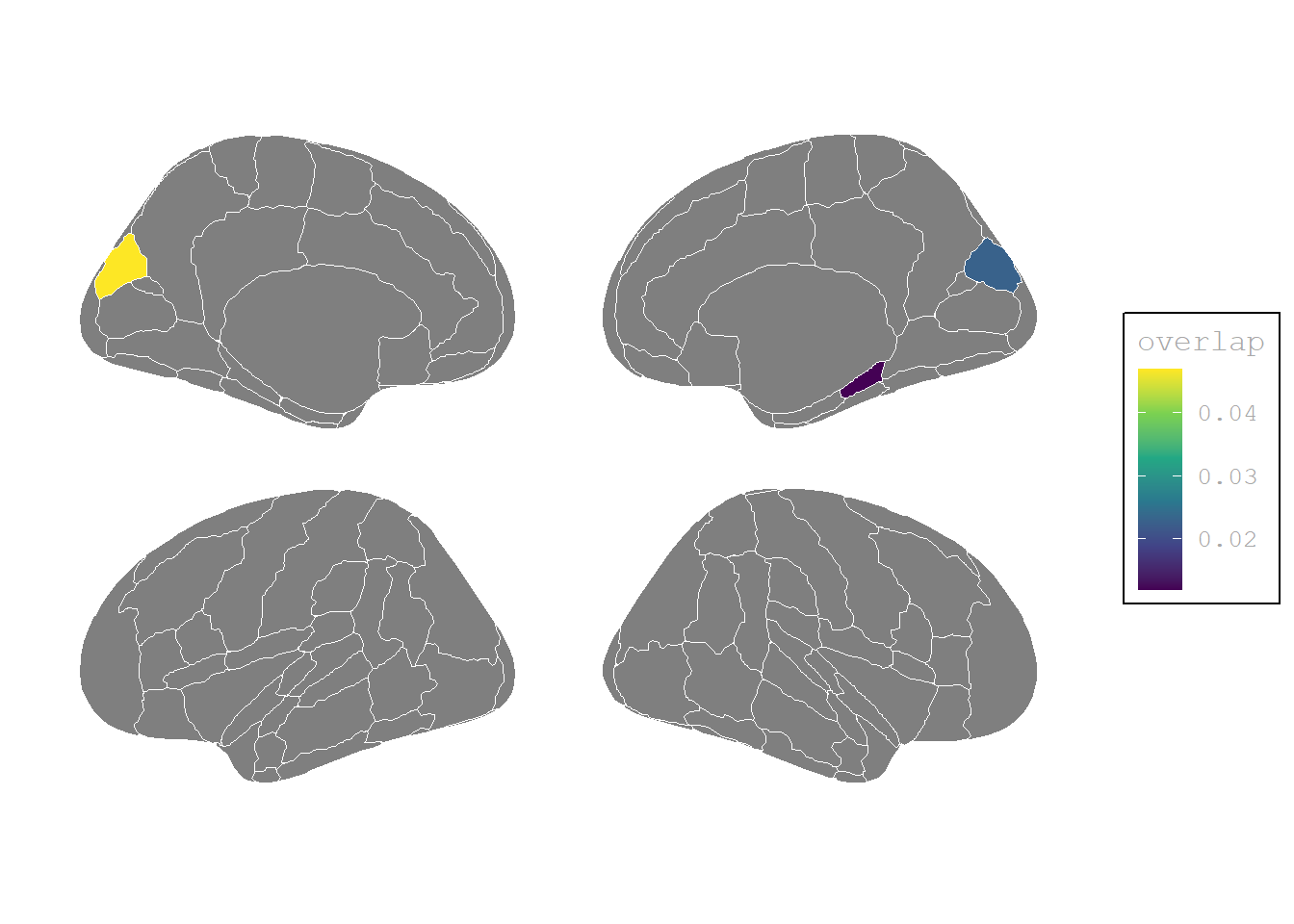

Activation barchart

Code

theme_set(theme_minimal())

# df_regio_abr %>% select(reg_abrv, persp) %>% 
#                  distinct() %>% 
#                  right_join(tab_4, by = c("reg_abrv" = "brain_region")) %>% 
#           filter(persp != "subcort") %>% 
#           mutate(rel_overlap = perc_overlap/100) %>% 
# # tab_4 %>% mutate(rel_overlap = perc_overlap/100) %>% 
#           ggplot(aes(x = reorder(reg_abrv, rel_overlap), 
#                      y = rel_overlap, fill = rel_overlap)) + 
#           geom_bar(stat = "identity") + 
#           scale_fill_viridis_c(option = "viridis", guide = "none", direction = -1) +
#           scale_y_continuous("different voxels", labels = scales::label_percent()) +
#           facet_grid(contrast~side, scales = "free", space = "free") +
#         # theme(axis.ticks.y = element_blank()) +
#           labs(x = "brain region") + 
#           theme(# text = element_text(size = 20),
#                 panel.spacing = unit(0.5, "cm")) +
#           coord_flip() 
#         # theme_minimal()

tab_4 %>% mutate(rel_overlap = perc_overlap/100) %>% 
          ggplot(aes(x = reorder(brain_region, rel_overlap), 
                     y = rel_overlap, fill = rel_overlap)) + 
          geom_bar(stat = "identity") + 
          scale_fill_viridis_c(option = "viridis", guide = "none", direction = 1) +
          scale_y_continuous("different voxels", labels = scales::label_percent()) +
          facet_grid(contrast~side, scales = "free", space = "free", drop = TRUE) +
        # theme(axis.ticks.y = element_blank()) +
          labs(x = "brain region") + 
          theme(# text = element_text(size = 20),
                panel.spacing = unit(0.5, "cm")) +
          coord_flip() -> vxl_chrt_d
vxl_chrt_d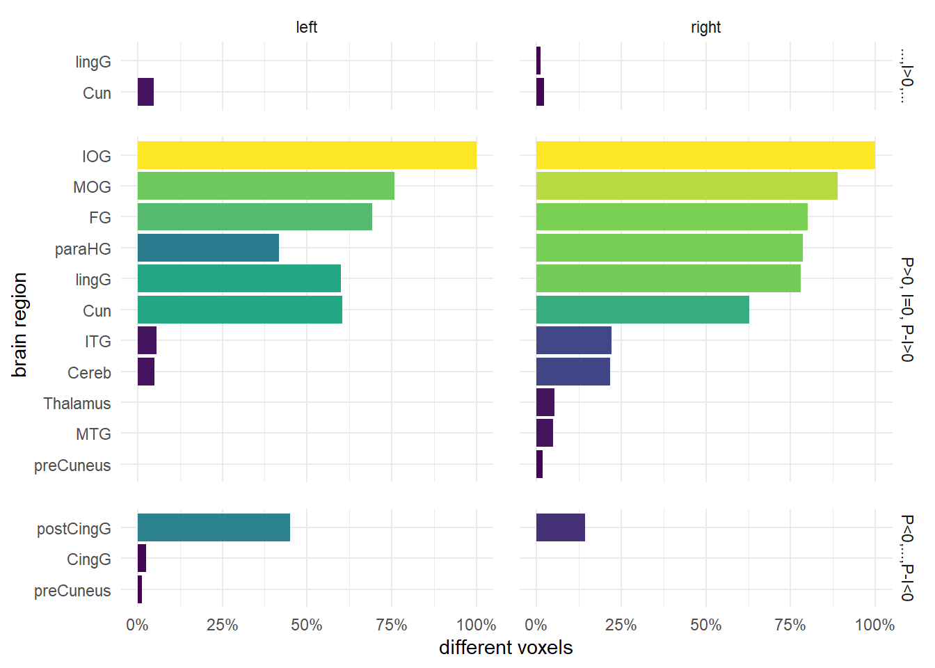

Table D voxels

Code

tab_4 %>% mutate(contrast = factor(contrast,
                 labels = c("P>0, I>0, P-I>0", "P>0, I=0, P-I>0", "P<0, I=0, P-I<0"))) %>% 
          pivot_wider(names_from = "side", 
                      values_from = c("perc_overlap", "D_voxels", "x", "y", "z")) %>% 
          relocate("D_voxels_left", .before = "perc_overlap_left") %>% 
          relocate("D_voxels_right", .before = "perc_overlap_right") %>% 
          relocate("y_left", .after = "x_left") %>%  
          relocate("z_left", .after = "y_left") -> tab_4_wide

df_regio_abr %>% select(c(reg_abrv, reg_name, persp)) %>% 
                 distinct() %>% 
                 right_join(tab_4_wide, by = c("reg_abrv" = "brain_region")) %>% 
                 mutate(brain_region = paste0(reg_name, " (", reg_abrv, ")")) %>%
               # filter(persp != "lateral") %>% 
                 select(-c(reg_name, persp, reg_abrv)) %>% 
# tab_4_wide %>% left_join(df_regio_abr, by = c("brain_region" = "reg_abrv")) %>% 
#                mutate(brain_region = paste0(reg_name, " (", brain_region, ")")) %>%
#                select(-c(reg_name, persp)) %>% 
               gt(rowname_col = "brain_region",
                  groupname_col = "contrast") %>% 
               tab_stubhead(label = "Contrast") %>% 
               tab_spanner(label = "left", 
                           columns = c(D_voxels_left, perc_overlap_left, x_left,    y_left, z_left)) %>% 
               tab_spanner(label = "right", 
                           columns = c(D_voxels_right, perc_overlap_right, x_right, y_right, z_right)) %>% 
               # tab_spanner(label = "left", 
               #             columns = c(x_left,    y_left, z_left)) %>% 
               # tab_spanner(label = "right", 
               #             columns = c(x_right,   y_right, z_right)) %>% 
               cols_label(D_voxels_left = "D voxels",
                          perc_overlap_left = "%",
                          D_voxels_right = "D voxels",
                          perc_overlap_right = "%",
                          x_left = "x", y_left = "y", z_left = "z",
                          x_right = "x ", y_right = "y ", z_right = "z ") %>% 
               cols_align(align = "center", columns = everything()) %>% 
               sub_missing() %>% 
               as_raw_html()

Contrast	right					left
Contrast	D voxels	%	x	y	z	D voxels	%	x	y	z
P>0, I=0, P-I>0
Inferior temporal gyrus (ITG)	9	22.2	42	-65	0	18	5.6	-46	-69	0
Middle temporal gyrus (MTG)	62	4.8	40	-70	12	—	—	—	—	—
Middle occipital gyrus (MOG)	90	88.9	33	-82	9	58	75.9	-30	-86	9
Inferior occipital gyrus (IOG)	23	100.0	38	-76	-4	43	100.0	-42	-79	-4
Parahippocampal gyrus (paraHG)	14	78.6	23	-49	-3	12	41.7	-27	-55	-5
Fusiform gyrus (FG)	15	80.0	25	-62	-9	13	69.2	-28	-60	-8
Lingual gyrus (lingG)	86	77.9	16	-77	3	45	60.0	-19	-76	-3
Precuneus (preCuneus)	121	1.7	24	-79	32	—	—	—	—	—
Cuneus (Cun)	86	62.8	18	-88	21	43	60.5	-19	-89	20
Thalamus (Thalamus)	95	5.3	17	-30	4	—	—	—	—	—
Cerebellum (Cereb)	46	21.7	21	-48	-10	41	4.9	-30	-49	-12
P<0, I=0, P-I<0
Posterior cingulate gyrus (postCingG)	14	14.3	2	-53	18	20	45.0	-4	-53	19
Precuneus (preCuneus)	—	—	—	—	—	159	1.3	-6	-55	26
Cingulate gyrus (CingG)	—	—	—	—	—	127	2.4	-3	-53	28
P>0, I>0, P-I>0
Lingual gyrus (lingG)	86	1.2	6	-85	-8	—	—	—	—	—
Cuneus (Cun)	86	2.3	16	-84	20	43	4.7	-6	-89	10

Shared voxels (S)

Code

tab_2 <- read_table(here("data", "neuro", "tab_2.txt"),
                    col_types = list(side = col_character(),
                                     brain_region = col_character(),
                                     perc_overlap = col_double(),
                                     S_voxels = col_character())) %>% 
         mutate(side = factor(side, levels = c("L", "R"), 
                              labels = c("left", "right")),
                brain_region = if_else(brain_region == "Claustrun", 
                                       "Claustrum", 
                                       brain_region), 
                brain_region = if_else(brain_region == "ling", 
                                       "lingG", 
                                       brain_region), 
                S_voxels = stringr::str_replace_all(S_voxels, "\\*|\\(|\\)", ""),
                S_voxels = as.numeric(S_voxels)) %>% 
         distinct()

# tab_2 %>% duplicated()

Plots

Code

theme_set(theme_brain2())

tab_2 %>% # left_join(df_regio_abr, by = c("brain_region" = "reg_abrv")) %>% 
          left_join(df_regio_abr2, by = c("brain_region" = "reg_abrv")) %>%
          rename(hemi = side) %>% 
        # mutate_at(scale, .vars = vars(C_voxels)) %>% 
          mutate(overlap = perc_overlap/100) %>% 
          select(-c(brain_region, # reg_name, 
                    perc_overlap)) %>% 
          filter(!is.na(region)) %>%
          ggplot() +
          scale_fill_viridis_c(option = "D", direction = 1)  +
          geom_brain(atlas = hoCort, # atlas = dk, 
                     color = "white",
                     position = position_brain(side ~ hemi),
                     mapping = aes(fill = overlap)) +
          labs(fill = "overlap") + 
          theme(# legend.position = "none",
                plot.background = element_blank())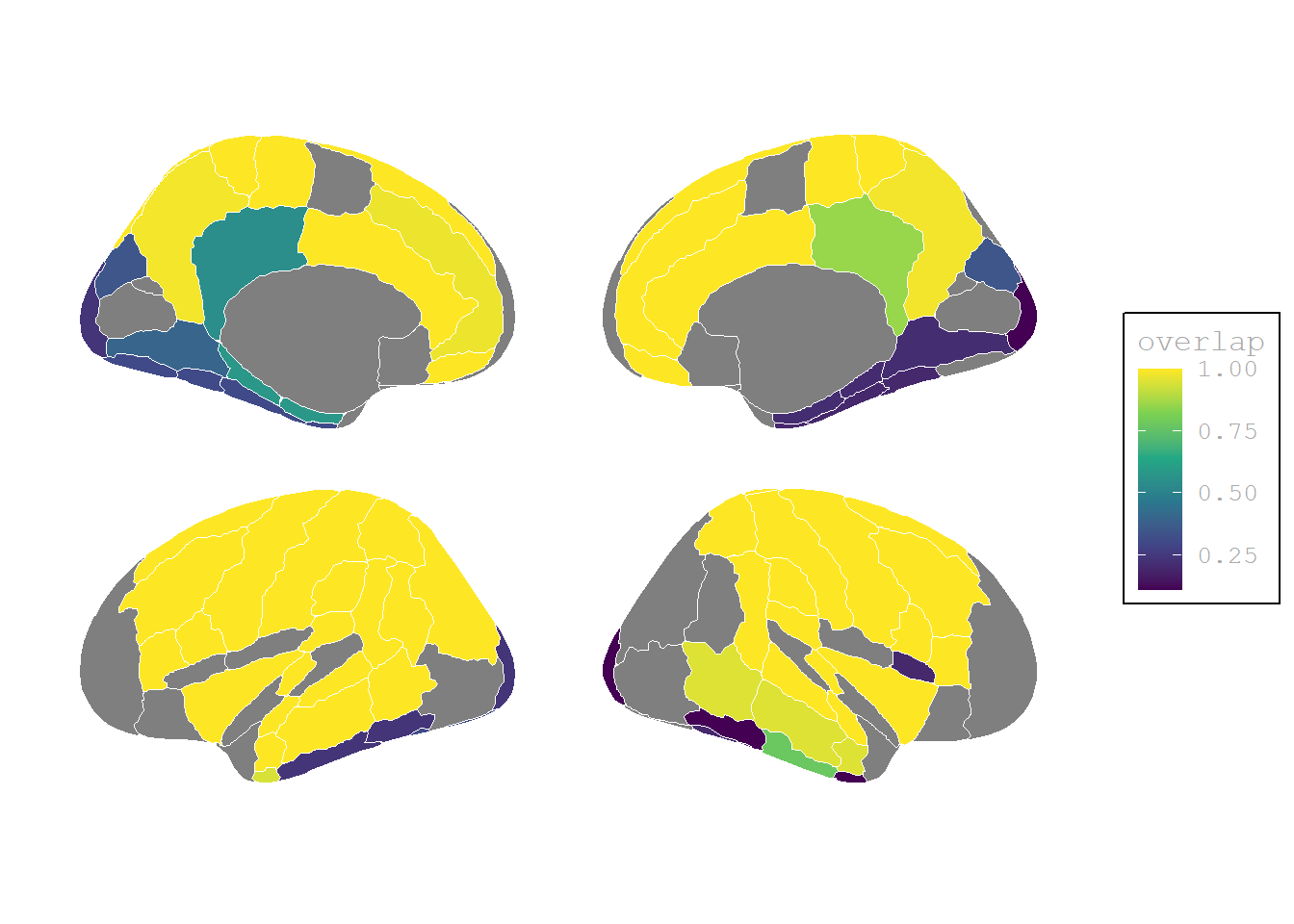

Activation barchart

Code

theme_set(theme_minimal())

# df_regio_abr %>% select(reg_abrv, persp) %>% 
#                  distinct() %>% 
#                  right_join(tab_2, by = c("reg_abrv" = "brain_region")) %>% 
#           filter(persp != "subcort") %>% 
#           mutate(rel_overlap = perc_overlap/100) %>% 
#           ggplot(aes(x = reorder(reg_abrv, rel_overlap), 
#                      y = rel_overlap, fill = rel_overlap)) + 
#           geom_bar(stat = "identity") + 
#           # scale_fill_viridis_c(option = "viridis", guide = "none", direction = -1) +
#           scale_fill_viridis_c(option = "D", guide = "none", direction = 1) +
#           scale_y_continuous("shared voxels", labels = scales::label_percent()) +
#           facet_grid(persp~side, scales = "free_y", space = "free_y") + 
#           theme(axis.ticks.y = element_blank()) +
#           labs(x = "brain region") + 
#           theme(# text = element_text(size = 20),
#                 panel.spacing = unit(0.5, "cm")) +
#           coord_flip()

tab_2 %>% mutate(rel_overlap = perc_overlap/100) %>% 
          ggplot(aes(x = reorder(brain_region, rel_overlap), 
                     y = rel_overlap, fill = rel_overlap)) + 
          geom_bar(stat = "identity") + 
          scale_fill_viridis_c(option = "viridis", guide = "none", direction = 1) +
          scale_y_continuous("shared voxels", labels = scales::label_percent()) +
          facet_grid(.~side, scales = "free", space = "free", drop = TRUE) +
        # theme(axis.ticks.y = element_blank()) +
          labs(x = "brain region") + 
          theme(# text = element_text(size = 20),
                panel.spacing = unit(0.5, "cm")) +
          coord_flip() -> vxl_chrt_s
vxl_chrt_s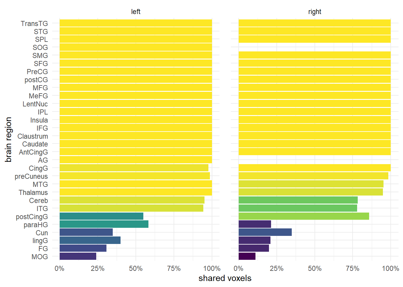

Table S voxels

Percentage of shared voxels (perc_overlap) and the total number of activated voxels (S_voxels = C+D voxels) for each region (brain_region) and side (side) of the brain:

Code

tab_2 %>% pivot_wider(names_from = "side", 
                      values_from = c("perc_overlap", "S_voxels")) %>% 
          relocate("S_voxels_left", .before = "perc_overlap_left") %>% 
          relocate("S_voxels_right", .before = "perc_overlap_right") -> tab_2_wide

df_regio_abr %>% select(c(reg_abrv, reg_name, persp)) %>% 
                 distinct() %>% 
                 right_join(tab_2_wide, by = c("reg_abrv" = "brain_region")) %>% 
                 mutate(brain_region = paste0(reg_name, " (", reg_abrv, ")")) %>%
               # filter(persp != "lateral") %>% 
                 select(-c(reg_name, persp, reg_abrv)) %>% 
                 gt(rowname_col = "brain_region") %>% 
                 tab_stubhead(label = "Region") %>% 
                 tab_spanner(label = "left", columns = c(S_voxels_left, perc_overlap_left)) %>% 
                 tab_spanner(label = "right", columns = c(S_voxels_right, perc_overlap_right)) %>% 
                 cols_label(S_voxels_left = "S voxels",
                            perc_overlap_left = "%",
                            S_voxels_right = "S voxels",
                            perc_overlap_right = "%") %>% 
                 sub_missing() %>% 
                 cols_align(align = "center", columns = everything()) %>% 
                 as_raw_html()

Region	left		right
Region	S voxels	%	S voxels	%
Inferior frontal gyrus (IFG)	241	100.0	146	100.0
Middle frontal gyrus (MFG)	325	100.0	250	100.0
Superior frontal gyrus (SFG)	93	100.0	88	100.0
Precentral gyrus (PreCG)	231	100.0	80	100.0
Postcentral gyrus (postCG)	157	100.0	31	100.0
Inferior parietal lobule (IPL)	206	100.0	91	100.0
Superior parietal lobule (SPL)	80	100.0	53	100.0
Angular gyrus (AG)	11	100.0	—	—
Supramarginal gurus (SMG)	47	100.0	15	100.0
Inferior temporal gyrus (ITG)	18	94.4	9	77.8
Middle temporal gyrus (MTG)	94	100.0	62	95.2
Superior temporal gyrus (STG)	226	100.0	173	100.0
Transverse temporal gyrus (TransTG)	18	100.0	20	100.0
Superior occipital gyrus (SOG)	2	100.0	—	—
Middle occipital gyrus (MOG)	58	24.1	90	11.1
Medial frontal gyrus (MeFG)	113	100.0	90	100.0
Insula (Insula)	99	100.0	87	100.0
Anterior cingulate gyrus (AntCingG)	30	100.0	13	100.0
Posterior cingulate gyrus (postCingG)	20	55.0	14	85.7
Parahippocampal gyrus (paraHG)	12	58.3	14	21.4
Fusiform gyrus (FG)	13	30.8	15	20.0
Lingual gyrus (lingG)	45	40.0	86	20.9
Precuneus (preCuneus)	159	98.7	121	98.3
Cuneus (Cun)	43	34.8	86	34.9
Lenticular nucleus (LentNuc)	102	100.0	55	100.0
Claustrum (Claustrum)	29	100.0	20	100.0
Thalamus (Thalamus)	114	100.0	95	94.7
Caudate nucleus (Caudate)	50	100.0	46	100.0
Cingulate gyrus (CingG)	127	97.6	108	100.0
Cerebellum (Cereb)	41	95.1	46	78.3

Literature

Brodman, K. (1909). Vergleichende Lokalisationslehre der Grosshirnrinde, in ihren Prinzipien dargestellt auf Grund des Zellenbaues. Barth Leipzig.

Flechsig, P. E. (1920). Anatomie des menschlichen Gehirns und Rückenmarks auf myelogenetischer Grundlage (Bd. 1). Thieme.

Ganis, G., Thompson, W. L., & Kosslyn, S. M. (2004). Brain areas underlying visual mental imagery and visual perception: an fMRI study. Cognitive Brain Research, 20(2), 226–241. https://doi.org/10.1016/j.cogbrainres.2004.02.012

Makris, N., Goldstein, J. M., Kennedy, D., Hodge, S. M., Caviness, V. S., Faraone, S. V., Tsuang, M. T., & Seidman, L. J. (2006). Decreased volume of left and total anterior insular lobule in schizophrenia. Schizophrenia research, 83(2-3), 155–171. https://doi.org/10.1016/j.schres.2005.11.020

Pijnenburg, R., Scholtens, L. H., Ardesch, D. J., Lange, S. C. de, Wei, Y., & Heuvel, M. P. van den. (2021). Myelo-and cytoarchitectonic microstructural and functional human cortical atlases reconstructed in common MRI space. NeuroImage, 239, 118274. https://doi.org/10.1016/j.neuroimage.2021.118274

Wickham, H. (2010). A layered grammar of graphics. Journal of Computational and Graphical Statistics, 19(1), 3–28. https://doi.org/doi.org/10.1198/jcgs.2009.07098

Fußnoten

some of the plots are used in a powerpoint-presentation dealing with the results described by Ganis et al. (2004)↩︎
In the paper the tables are presented in a different order, but didactically the order listed here makes more sense in my opinion.↩︎